Supervised Learning 1

Book

This IPython notebook follows the book Introduction to Machine Learning with Python by Andreas Mueller and Sarah Guido and uses material from its github repository and from the working files of the training course Advanced Machine Learning with scikit-learn. Excerpts taken from the book are displayed in italic letters.

The contents of this Jupyter notebook corresponds in the book Introduction to Machine Learning with Python to:

Chapter 1 “Introduction”: p. 1 to 24
Chapter 2 “Supervised Learning”: p. 25 to 44

Python

Packages provided by Anaconda

To (re-)install the scikit-learn package, the pandas package or other packages provided by the Anconda Repository in use the following commands in the Anaconda Command Prompt :

conda install scikit-learn
conda install pandas
conda install <package-name>

import pandas as pd
import matplotlib.pyplot as plt
import numpy as np

mglearn

Um das Python-Paket mglearn zum Buch Introduction to Machine Learning with Python: A Guide for Data Scientists importieren zu können, installieren Sie im Anaconda Command Prompt das Paket mglearn mit dem Befehl pip install mglearn.

# Danach sollte der folgende Import des Pakets funktionieren:
import mglearn

Deactivate Warnings

if 0:
    import warnings
    warnings.filterwarnings("ignore")

Why Machine Learning?

Objectives:

decision support: prediction; Spam filter; classification; finding similarities; pattern recognition; recommendation systems; detecting faces, letters and numbers etc.
finding correlations: positive, negative or zero. Attention: Correlation is not causality!
feature extraction: dimensionality reduction

Expert-designed rules to make decisions have disadvantages (logic is specific to a single domain, deep human understanding required) compared to rules extracted automatically from data.

Problems that machine learning can solve

supervised learning examples:
- Identifying the zip code from handwritten digits on an envelope
- Determining whether a tumor is benign based on a medical image
- Detecting fraudulent activity in credit card transactions
unsupervised learning examples:
- Identifying topics in a set of blog posts
- Segmenting customers into groups with similar preferences
- Detecting abnormal access patterns to a website

Knowing your task and knowing your data

What question(s) am I trying to answer? Do I think the data collected can answer that question?
What is the best way to phrase my question(s) as a machine learning problem?
Have I collected enough data to represent the problem I want to solve?
What features of the data did I extract, and will these enable the right predictions?
How will I measure success in my application?
How will the machine learning solution interact with other parts of my research or business product?

A First Application: Classifying iris species

Meet the data

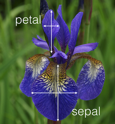
As an example of a simple dataset, we’re going to take a look at the iris flower data set stored by scikit-learn. The data consists of measurements of three different species of irises. There are three species of iris in the dataset:

Iris Setosa:

Iris Versicolor:

Iris Virginica:

Data Structure

Most machine learning algorithms implemented in scikit-learn expect data to be stored in a two-dimensional array or matrix:

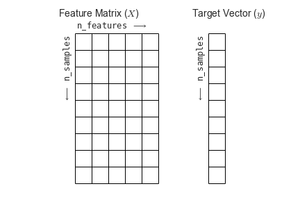
The figure is taken from the Python Data Science Handbook.

from sklearn.datasets import load_iris
iris_dataset = load_iris()

# print(iris_dataset['DESCR'])

iris_dataset.keys()

dict_keys(['data', 'target', 'frame', 'target_names', 'DESCR', 'feature_names', 'filename', 'data_module'])

print(f"Target names: {iris_dataset['target_names']}")

Target names: ['setosa' 'versicolor' 'virginica']

print(f"Feature names: {iris_dataset['feature_names']}")

Feature names: ['sepal length (cm)', 'sepal width (cm)', 'petal length (cm)', 'petal width (cm)']

print(f"Type of data: {type(iris_dataset['data'])}")

Type of data: <class 'numpy.ndarray'>

print(f"Shape of data: {iris_dataset['data'].shape}")

Shape of data: (150, 4)

print(f"First five rows of data:\n{iris_dataset['data'][:5]}")

First five rows of data:
[[5.1 3.5 1.4 0.2]
 [4.9 3.  1.4 0.2]
 [4.7 3.2 1.3 0.2]
 [4.6 3.1 1.5 0.2]
 [5.  3.6 1.4 0.2]]

print(f"Type of target: {type(iris_dataset['target'])}")

Type of target: <class 'numpy.ndarray'>

print(f"Shape of target: {iris_dataset['target'].shape}")

Shape of target: (150,)

print(f"Target:\n{iris_dataset['target']}")

Target:
[0 0 0 0 0 0 0 0 0 0 0 0 0 0 0 0 0 0 0 0 0 0 0 0 0 0 0 0 0 0 0 0 0 0 0 0 0
 0 0 0 0 0 0 0 0 0 0 0 0 0 1 1 1 1 1 1 1 1 1 1 1 1 1 1 1 1 1 1 1 1 1 1 1 1
 1 1 1 1 1 1 1 1 1 1 1 1 1 1 1 1 1 1 1 1 1 1 1 1 1 1 2 2 2 2 2 2 2 2 2 2 2
 2 2 2 2 2 2 2 2 2 2 2 2 2 2 2 2 2 2 2 2 2 2 2 2 2 2 2 2 2 2 2 2 2 2 2 2 2
 2 2]

First things first: Look at your data

# label the columns using the strings in iris_dataset.feature_names
iris_dataframe = pd.DataFrame(iris_dataset['data'], 
                              columns=iris_dataset['feature_names'])
iris_dataframe.head()

	sepal length (cm)	sepal width (cm)	petal length (cm)	petal width (cm)
0	5.1	3.5	1.4	0.2
1	4.9	3.0	1.4	0.2
2	4.7	3.2	1.3	0.2
3	4.6	3.1	1.5	0.2
4	5.0	3.6	1.4	0.2

# create a scatter matrix from the dataframe, color by y_train
pd.plotting.scatter_matrix(iris_dataframe, c=iris_dataset['target'],
                           figsize=(12, 12), marker='o', 
                           hist_kwds={'bins': 20}, s=60, alpha=.8, 
                           cmap=plt.get_cmap('coolwarm'));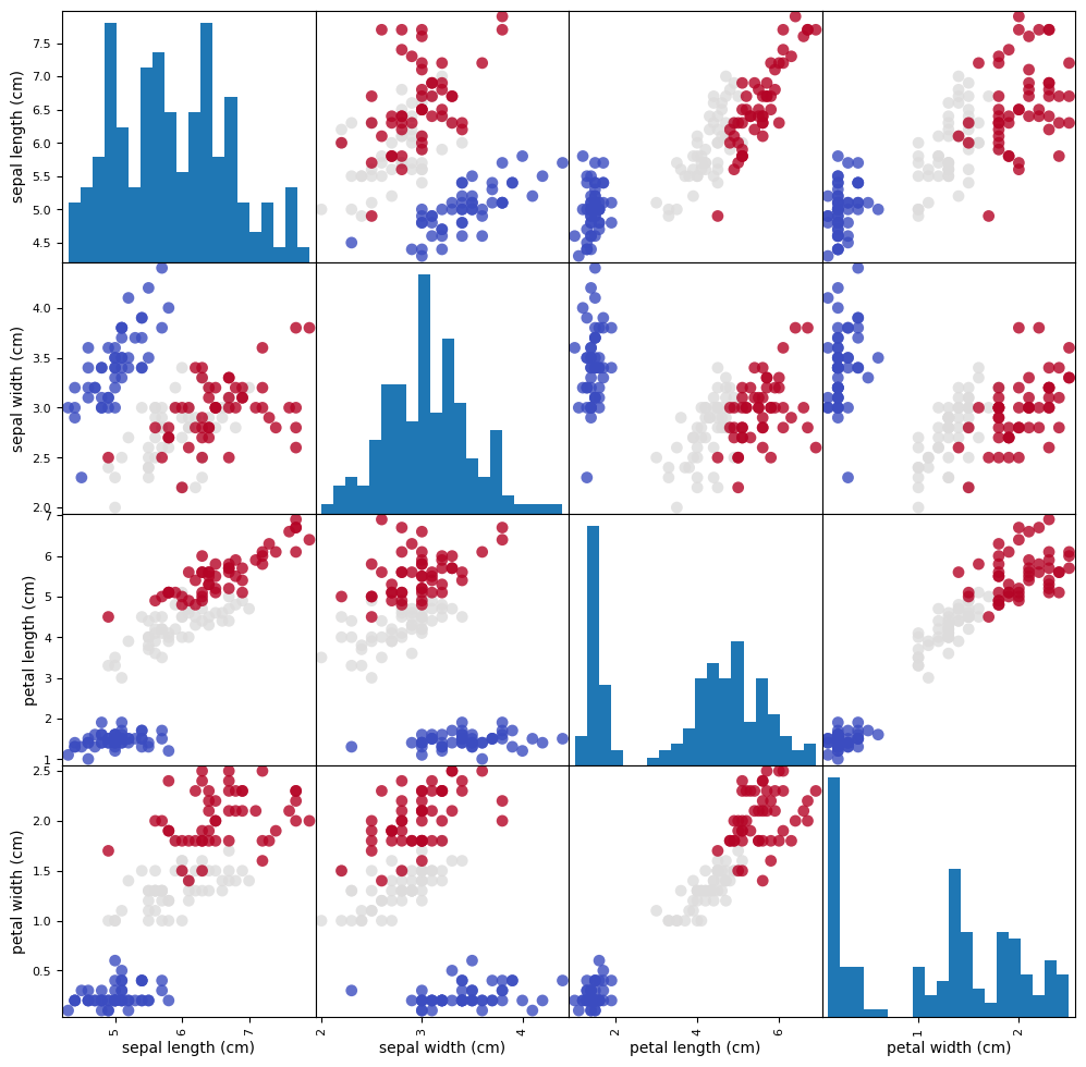

Correlation Matrix

See literature and for example Wikipedia: Korrelationskoeffizient.

iris_dataframe.corr()

	sepal length (cm)	sepal width (cm)	petal length (cm)	petal width (cm)
sepal length (cm)	1.000000	-0.117570	0.871754	0.817941
sepal width (cm)	-0.117570	1.000000	-0.428440	-0.366126
petal length (cm)	0.871754	-0.428440	1.000000	0.962865
petal width (cm)	0.817941	-0.366126	0.962865	1.000000

Measuring Success: Training and testing data

from sklearn.model_selection import train_test_split
X_train, X_test, y_train, y_test = train_test_split(
    iris_dataset['data'], iris_dataset['target'], random_state=0)

print(f"X_train shape: {X_train.shape}")
print(f"y_train shape: {y_train.shape}")

X_train shape: (112, 4)
y_train shape: (112,)

print(f"X_test shape: {X_test.shape}")
print(f"y_test shape: {y_test.shape}")

X_test shape: (38, 4)
y_test shape: (38,)

Building your first model: k nearest neighbors

from sklearn.neighbors import KNeighborsClassifier

knn = KNeighborsClassifier(n_neighbors=1)

knn.fit(X_train, y_train)

KNeighborsClassifier(n_neighbors=1)

In a Jupyter environment, please rerun this cell to show the HTML representation or trust the notebook.
On GitHub, the HTML representation is unable to render, please try loading this page with nbviewer.org.

Making predictions

X_new = np.array([[5, 2.9, 1, 0.2]])
print(f"X_new.shape: {X_new.shape}")

X_new.shape: (1, 4)

prediction = knn.predict(X_new)
print(f"Prediction: {prediction}")
print(f"Predicted target name: {iris_dataset['target_names'][prediction]}")

Prediction: [0]
Predicted target name: ['setosa']

Evaluating the model

y_pred = knn.predict(X_test)
print(f"Test set predictions:\n {y_pred}")

Test set predictions:
 [2 1 0 2 0 2 0 1 1 1 2 1 1 1 1 0 1 1 0 0 2 1 0 0 2 0 0 1 1 0 2 1 0 2 2 1 0
 2]

print(f"Test set score: {np.mean(y_pred == y_test):.12f}")

Test set score: 0.973684210526

print(f"Test set score: {knn.score(X_test, y_test):.12f}")

Test set score: 0.973684210526

Summary

X_train, X_test, y_train, y_test = train_test_split(
    iris_dataset['data'], iris_dataset['target'], random_state=0)

knn = KNeighborsClassifier(n_neighbors=1)
knn.fit(X_train, y_train)

print(f"Test set score: {knn.score(X_test, y_test):.2f}")

Test set score: 0.97

Zusammenhang vs. Kausalität

Typen von Kausalität

Fall 1: \(A \Rightarrow B\) oder \(B \Leftarrow A\), aus \(A\) folgt \(B\), \(A\) verursacht \(B\), Beispiele:

viel Essen \(\Rightarrow\) dick sein
Stückpreis und Qualität \(\Rightarrow\) Umsatz

Eine einseitige Einflußnahme ist möglich.

Fall 2: \(A \Leftrightarrow B\) Beispiel: \(U \Leftrightarrow I\) im Ohmschen Gesetz

Die gegenseitige Einflußnahme möglich.

Fall 3: \(A \Leftarrow C \Rightarrow B\) Beispiele:

mit einem Schuh schlafen \(\Leftarrow C \Rightarrow\) Aufwachen mit Kopfweh
in einem Land: CO\(_2\)-Ausstoß \(\Leftarrow C \Rightarrow\) Fettleibigkeit
Eiscremekonsum \(\Leftarrow C \Rightarrow\) Ertrinken von Kindern

Eine Einflußnahme von \(A\) auf \(B\) oder umgekehrt ist nicht möglich.

Zusammenhang

In allen drei obigen Fällen gibt es einen Zusammenhang zwischen \(A\) und \(B\), geschrieben als \(A \sim B\).

Achtung! Nur weil keine Kausalität bekannt ist, bedeutet das nicht zwingend, dass ein bestehender Zusammenhang nicht verwendet werden kann, um nützliche Vorhersagen zu treffen.

Classification and Regression

In classification, the goal is to predict a class label, which is a choice from a predefined list of possibilities. Examples:

binary classification: classifying emails as either spam or not spam
multiclass classification: iris example, language of a website

For regression tasks, the goal is to predict a continuous number. Examples:

persons’ annual income from their education, their age, and where they live
yield of a corn farm given attributes such as previous yields, weather, and number of employees working on the farm

Generalization, Overfitting and Underfitting

Beispiel: potentielle Schiffskäufer, Buch Seite 27f.

In supervised learning, we want to build a model on the training data and then be able to make accurate predictions on new, unseen data that has the same characteristics as the training set that we used. If a model is able to make accurate predictions on unseen data, we say it is able to generalize from the training set to the test set.

Building a model that is too complex for the amount of information we have, is called overfitting.
Choosing too simple a model is called underfitting.

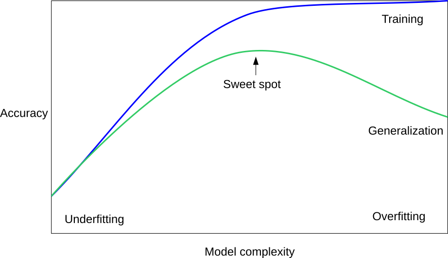
The larger variety of data points your dataset contains, the more complex a model you can use without overfitting.

Examples of Datasets

Synthetic Sample Datasets

Zwei-dimensional, um grafische Darstellung zu erleichtern.

# Classification:

X, y = mglearn.datasets.make_forge()

print(f"X.shape: {X.shape}")

plt.figure(figsize=(8,6))
mglearn.discrete_scatter(X[:, 0], X[:, 1], y)
plt.legend(["class 0", "class 1"], loc=4)
plt.xlabel("first feature")
plt.ylabel("second feature")
plt.grid(True)

X.shape: (26, 2)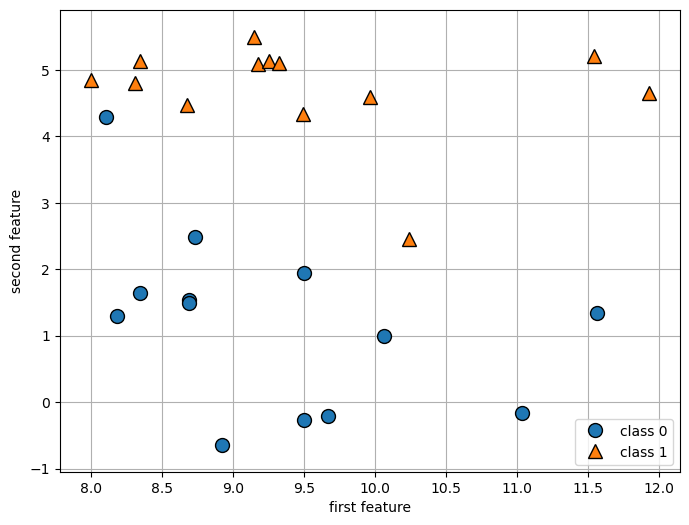

# Regression:

X, y = mglearn.datasets.make_wave(n_samples=40)

plt.figure(figsize=(8,6))
plt.plot(X, y, 'o')
plt.ylim(-3, 3)
plt.xlabel("Feature")
plt.ylabel("Target")
plt.grid(True)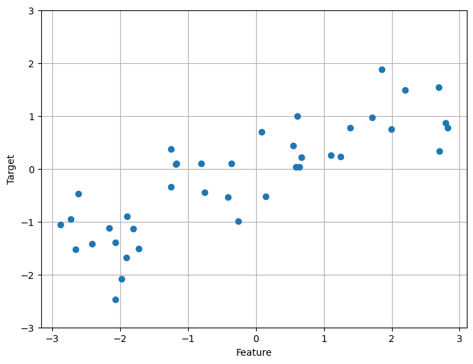

Real Sample Datasets

Breast Cancer Wisconsin (Diagnostic) Dataset

from sklearn.datasets import load_breast_cancer

cancer = load_breast_cancer()
cancer.keys()

dict_keys(['data', 'target', 'frame', 'target_names', 'DESCR', 'feature_names', 'filename', 'data_module'])

# print(cancer.DESCR)

cancer.data.shape

(569, 30)

# Class Distribution: 212 - Malignant, 357 - Benign
print(cancer.target_names)
print(np.bincount(cancer.target))

['malignant' 'benign']
[212 357]

sum(cancer.target == 0)

cancer.feature_names

array(['mean radius', 'mean texture', 'mean perimeter', 'mean area',
       'mean smoothness', 'mean compactness', 'mean concavity',
       'mean concave points', 'mean symmetry', 'mean fractal dimension',
       'radius error', 'texture error', 'perimeter error', 'area error',
       'smoothness error', 'compactness error', 'concavity error',
       'concave points error', 'symmetry error',
       'fractal dimension error', 'worst radius', 'worst texture',
       'worst perimeter', 'worst area', 'worst smoothness',
       'worst compactness', 'worst concavity', 'worst concave points',
       'worst symmetry', 'worst fractal dimension'], dtype='<U23')

Boston House Prices Dataset

# from sklearn.datasets import load_boston
# boston = load_boston()
# print(boston.DESCR)
# X, y = load_boston(return_X_y=True)

data_url = "http://lib.stat.cmu.edu/datasets/boston"
raw_df = pd.read_csv(data_url, sep="\s+", skiprows=22, header=None)
X = np.hstack([raw_df.values[::2, :], raw_df.values[1::2, :2]])
y = raw_df.values[1::2, 2]

print(X.shape)
print(y.shape)

(506, 13)
(506,)

# X, y = mglearn.datasets.load_extended_boston()
# print(X.shape)
# print(y.shape)

k-Neighbors Classification

Grafische Darstellungen

mglearn.plots.plot_knn_classification(n_neighbors=1)
plt.axis('equal');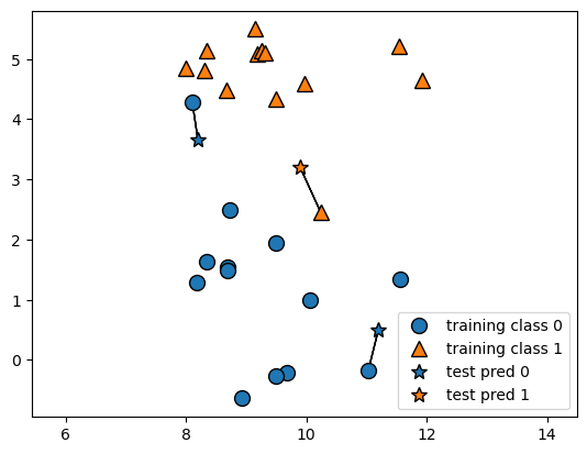

mglearn.plots.plot_knn_classification(n_neighbors=3)
plt.axis('equal');

Implementierung des Algorithmus

from sklearn.model_selection import train_test_split
X, y = mglearn.datasets.make_forge()

X_train, X_test, y_train, y_test = train_test_split(X, y, random_state=0)

from sklearn.neighbors import KNeighborsClassifier

clf = KNeighborsClassifier(n_neighbors=3)

clf.fit(X_train, y_train)

KNeighborsClassifier(n_neighbors=3)

print(f"Test set predictions: {clf.predict(X_test)}")

Test set predictions: [1 0 1 0 1 0 0]

print(f"Test set accuracy: {clf.score(X_test, y_test):.2f}")

Test set accuracy: 0.86

Analyzing KNeighborsClassifier

plt.figure(figsize=(12,4))

plt.subplot(1,3,1)
n_neighbors = 1
clf = KNeighborsClassifier(n_neighbors=n_neighbors).fit(X, y)
mglearn.plots.plot_2d_separator(clf, X, fill=True, eps=0.5, alpha=.4)
mglearn.discrete_scatter(X[:, 0], X[:, 1], y)
plt.title(f"{n_neighbors} neighbor(s)")
plt.xlabel("feature 0")
plt.ylabel("feature 1")

plt.subplot(1,3,2)
n_neighbors = 3
clf = KNeighborsClassifier(n_neighbors=n_neighbors).fit(X, y)
mglearn.plots.plot_2d_separator(clf, X, fill=True, eps=0.5, alpha=.4)
mglearn.discrete_scatter(X[:, 0], X[:, 1], y)
plt.title(f"{n_neighbors} neighbor(s)")
plt.xlabel("feature 0")
plt.ylabel("feature 1")

plt.subplot(1,3,3)
n_neighbors = 9
clf = KNeighborsClassifier(n_neighbors=n_neighbors).fit(X, y)
mglearn.plots.plot_2d_separator(clf, X, fill=True, eps=0.5, alpha=.4)
mglearn.discrete_scatter(X[:, 0], X[:, 1], y)
plt.title(f"{n_neighbors} neighbor(s)")
plt.xlabel("feature 0")
plt.ylabel("feature 1");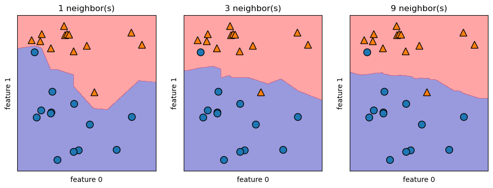

k-Neighbors Regression

Grafische Darstellungen

mglearn.plots.plot_knn_regression(n_neighbors=1)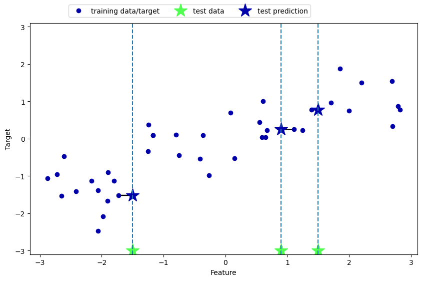

mglearn.plots.plot_knn_regression(n_neighbors=3)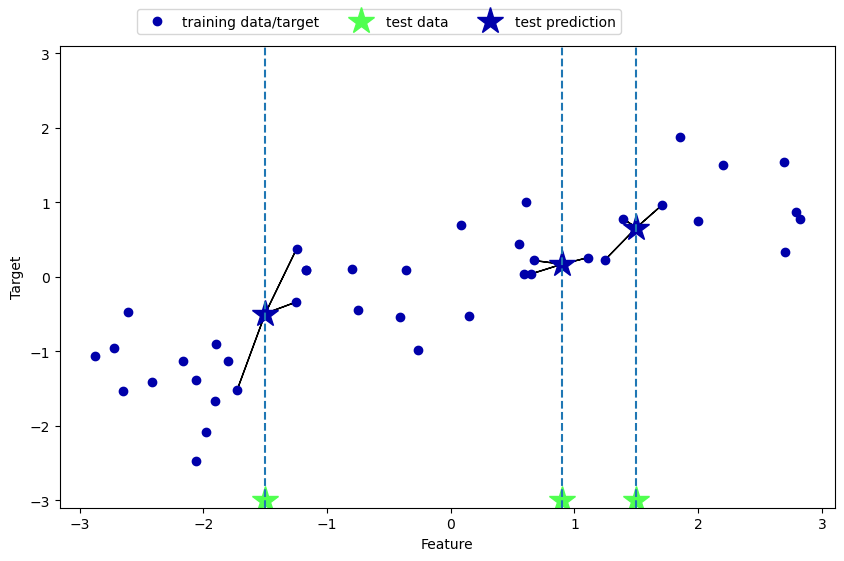

Implementierung des Algorithmus

# import KNeighborsRegressor function:
from sklearn.neighbors import KNeighborsRegressor

# load data:
X, y = mglearn.datasets.make_wave(n_samples=40)

# split the wave dataset into a training and a test set:
X_train, X_test, y_train, y_test = train_test_split(X, y, random_state=0)

# Instantiate the model, set the number of neighbors to consider to 3:
reg = KNeighborsRegressor(n_neighbors=3)

# Fit the model using the training data and training targets:
reg.fit(X_train, y_train)

KNeighborsRegressor(n_neighbors=3)

print(f"Test set predictions:\n{reg.predict(X_test)}")

Test set predictions:
[-0.05396539  0.35686046  1.13671923 -1.89415682 -1.13881398 -1.63113382
  0.35686046  0.91241374 -0.44680446 -1.13881398]

print(f"Test set R^2: {reg.score(X_test, y_test):.2f}")

Test set R^2: 0.83

k-Neighbors - strengths, weaknesses and parameters

Two important parameters to the KNeighbors classifier: the number of neighbors and how you measure distance between data points.
Building the nearest neighbors model is usually very fast, but when your training set is very large (either in number of features or in number of samples) prediction can be slow. When using the k-NN algorithm, it’s important to preprocess your data (see Chapter 3).
So, while the nearest k-neighbors algorithm is easy to understand, it is not often used in practice, due to prediction being slow and its inability to handle many features. The method we discuss next has neither of these drawbacks.
Weiterer Nachteil: Extrapolation nicht möglich.