import pandas as pd
import matplotlib.pyplot as plt
import numpy as np
import mglearnÜbung 4
Clustering und GridsearchCV
Python
from sklearn.datasets import load_iris

from sklearn.model_selection import train_test_split

from sklearn.neighbors import KNeighborsRegressor
from sklearn.linear_model import LinearRegression
from sklearn.linear_model import Ridge
from sklearn.linear_model import Lasso
from sklearn.linear_model import LogisticRegression
from sklearn.svm          import LinearSVC
from sklearn.tree import DecisionTreeClassifier
from sklearn.ensemble import RandomForestClassifier
from sklearn.ensemble import GradientBoostingClassifier
from sklearn.cluster  import KMeans
from sklearn.cluster import DBSCAN
from sklearn.preprocessing import PolynomialFeatures
from sklearn.feature_selection import SelectFromModel
from sklearn.feature_selection import RFE

from scipy.cluster.hierarchy import dendrogram, ward
# set default values for all plotting:
size=12
plt.rcParams['axes.labelsize'] = size
plt.rcParams['xtick.labelsize'] = size
plt.rcParams['ytick.labelsize'] = size
plt.rcParams['legend.fontsize'] = size
plt.rcParams['figure.figsize'] = (6.29, 6/10*6.29)
plt.rcParams['lines.linewidth'] = 1
plt.rcParams['axes.grid'] = True
# print(plt.rcParams)
# import locale # should you want german notation for numbers, then use the locale package
# locale.setlocale(locale.LC_ALL, "deu_deu")
# plt.rcParams['axes.formatter.use_locale'] = True
# Stylefile
# plt.style.use('C:/Users/edel/Documents/Python Scripts/Stylefile/custom_figure_style.mplstyle')Clustering
Aufgabe 1: Zusätzliche Features
Untersuchen Sie die moons-Daten:
- Klassifizieren Sie den Datensatz zunächst mittels einer logistischen Regression
- Überprüfen Sie nun, ob sich mit Hilfe der kMeans-Clustering Methode die zusätzlichen Features Clusterzugehörigkeit und Distanzen einsetzen lassen, um einen höheren Score zu erzielen.
- Ineinander verwickelte Cluster lassen sich mit dem DBScan-Clustering Algorithmus eindeutig clustern. Optimieren Sie diesen, um die beiden Cluster eindeutig zu identifizieren.
from sklearn.datasets import make_moons

X, y = make_moons(n_samples=200, noise=0.05, random_state=0)
Lösung:
X_train, X_test, y_train, y_test = train_test_split(X, y, random_state=0) #0

logreg = LogisticRegression().fit(X_train, y_train)

plt.figure()
mglearn.plots.plot_2d_separator(logreg, X, fill=False, eps=0.5, alpha=.7)
mglearn.discrete_scatter(X_train[:, 0], X_train[:, 1], y_train);

print("Training set score: {:.3f}".format(logreg.score(X_train, y_train)))
print("Test     set score: {:.3f}".format(logreg.score(X_test,  y_test)))
Training set score: 0.867
Test set score: 0.880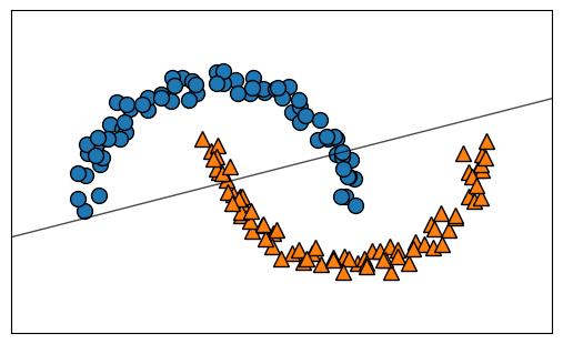
n_clust=10
kmeans = KMeans(n_clusters=n_clust, random_state=0,n_init=10)
kmeans.fit(X_train)

y_train_pred = kmeans.predict(X_train)
X_train_dist = kmeans.transform(X_train)
X_train_enhanced = np.hstack( (X_train, y_train_pred.reshape(-1,1), X_train_dist) )

y_test_pred  = kmeans.predict(X_test)
X_test_dist  = kmeans.transform(X_test)
X_test_enhanced  = np.hstack( (X_test , y_test_pred.reshape(-1,1) , X_test_dist ) )

logreg = LogisticRegression().fit(X_train_enhanced, y_train)

print("Training set score: {:.3f}".format(logreg.score(X_train_enhanced, y_train)))
print("Test     set score: {:.3f}".format(logreg.score(X_test_enhanced,  y_test)))
Training set score: 0.940
Test set score: 0.960import matplotlib.cm as cm
cluster_labels=kmeans.predict(X)
colors = cm.Accent(cluster_labels.astype(float) / n_clust)
plt.figure()
plt.scatter(
X[:, 0], X[:, 1], marker=".", s=80, lw=0, alpha=0.7, c=colors, edgecolor="k"
)
# Labeling the clusters
centers = kmeans.cluster_centers_
# Draw white circles at cluster centers
plt.scatter(
centers[:, 0],
centers[:, 1],
marker="o",
c="white",
alpha=1,
s=200,
edgecolor="k",
)
for i, c in enumerate(centers):
plt.scatter(c[0], c[1], marker="$%d$" % i, alpha=1, s=50, edgecolor="k")
plt.tight_layout()
plt.xticks([])
plt.yticks([])
plt.grid(False)
dbscan = DBSCAN(eps=.3,min_samples=2)
cluster_labels=dbscan.fit(X).labels_
#print(np.unique(cluster_labels))
n_clust=len(np.unique(cluster_labels))
#print(cluster_labels)
colors = cm.Accent(cluster_labels.astype(float)/n_clust)


plt.figure()
plt.scatter(
    X[:, 0], X[:, 1], marker=".", s=80, lw=0, alpha=0.7, c=colors, edgecolor="k"
)
plt.tight_layout()
plt.xticks([])
plt.yticks([])
plt.grid(False)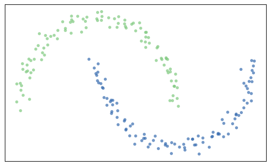
Aufgabe 2: 24h-Strompreise
Clustern Sie die 24h-Strompreise der Datei dshistory2013.xls:
- Erstellen Sie ein Dendrogramm zur Auswahl der Clusteranzahl.
- Vergleichen Sie Ihr Ergebnis mit einem Elbow-Plot zur Auswahl der passenden Clusteranzahl.
- Stellen Sie die Clusterzentren und die Clustermitglieder graphisch dar.
- Untersuchen Sie, ob es einen Zusammenhang zum Wochentag gibt.
price = pd.read_excel('daten/dshistory2013.xls', sheet_name='Price (EUR)',
                      index_col=0, skiprows=1)

# Preprocessing:
price.sort_index(inplace=True)
price = price.loc['2013-01-01':'2013-12-31']
price = price.iloc[:,:24]
price.loc['2013-10-27','hEXA02'] = (6.74 + 4.25)/2
price.loc['2013-03-31','hEXA03'] = 22
price = price.astype(float)
price.head(3)| hEXA01 | hEXA02 | hEXA03 | hEXA04 | hEXA05 | hEXA06 | hEXA07 | hEXA08 | hEXA09 | hEXA10 | ... | hEXA15 | hEXA16 | hEXA17 | hEXA18 | hEXA19 | hEXA20 | hEXA21 | hEXA22 | hEXA23 | hEXA24 | |
|---|---|---|---|---|---|---|---|---|---|---|---|---|---|---|---|---|---|---|---|---|---|
| Delivery Date | |||||||||||||||||||||
| 2013-01-01 | 1.39 | 0.01 | 0.01 | 0.01 | 0.01 | 0.01 | 0.01 | 0.01 | 0.01 | 8.07 | ... | 14.70 | 15.76 | 20.93 | 31.93 | 35.34 | 30.07 | 30.30 | 20.07 | 22.18 | 17.09 |
| 2013-01-02 | 10.43 | 1.93 | 0.01 | 0.01 | 0.01 | 12.51 | 24.43 | 34.43 | 35.00 | 36.43 | ... | 38.93 | 40.93 | 45.43 | 53.43 | 53.42 | 50.00 | 41.43 | 38.22 | 34.43 | 27.43 |
| 2013-01-03 | 25.43 | 15.56 | 14.60 | 11.66 | 12.18 | 17.81 | 34.32 | 43.68 | 44.43 | 42.99 | ... | 38.18 | 40.46 | 46.21 | 51.90 | 51.16 | 47.23 | 38.93 | 34.21 | 32.68 | 24.92 |
3 rows × 24 columns
Lösung:
X = price.values
X.shape
(365, 24)linkage_array = ward(X)
plt.figure()
dendrogram(linkage_array)
plt.xticks([])
plt.tight_layout()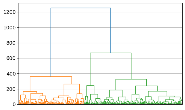
distortions = []
for k in range(1,21):
    kmeanModel = KMeans(n_clusters=k,n_init=10)
    kmeanModel.fit(X)
distortions.append(kmeanModel.inertia_)n_clust=np.arange(1,21,1)
plt.figure()
plt.plot(n_clust,distortions,color='red',ls='dashed',marker='.')
plt.xlim(0,20)
plt.xticks(np.arange(1,21,1))
plt.xlabel('Clusteranzahl')
plt.ylabel('Distortions') #Summe der quadrierten Abstände aller Punkte eines Clusters zum Zentrum des Clusters
plt.tight_layout()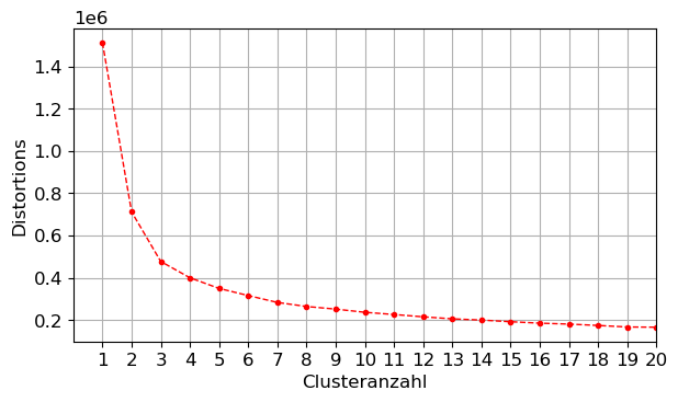
n = 3
kmeans = KMeans(n_clusters=n, n_init='auto')
kmeans.fit(X)

cluster = kmeans.labels_
day = price.index.dayofweek # The day of the week with Monday=0, Sunday=6plt.figure(figsize=(15, 10))
for k in range(n):
plt.subplot(2, n, k+1)
plt.plot(kmeans.cluster_centers_[k],'-b', linewidth=3)
plt.plot(X[cluster == k,:].T, alpha=0.1, color='b');
plt.title(f'Cluster {k+1}')
plt.xlabel('Stunde des Tages')
plt.ylim(-20, 110)
plt.grid(True)
plt.subplot(2, n, n + k+1)
data = day[cluster == k]
bins = np.arange(0, 8)
plt.hist(data, bins=bins, alpha=0.75, align='left', rwidth=0.9)
plt.title(f'Cluster {k+1}')
plt.xlabel('Wochentag')
plt.xlim(-1,7)
plt.ylim(0, 45)
plt.grid(True)
plt.tight_layout()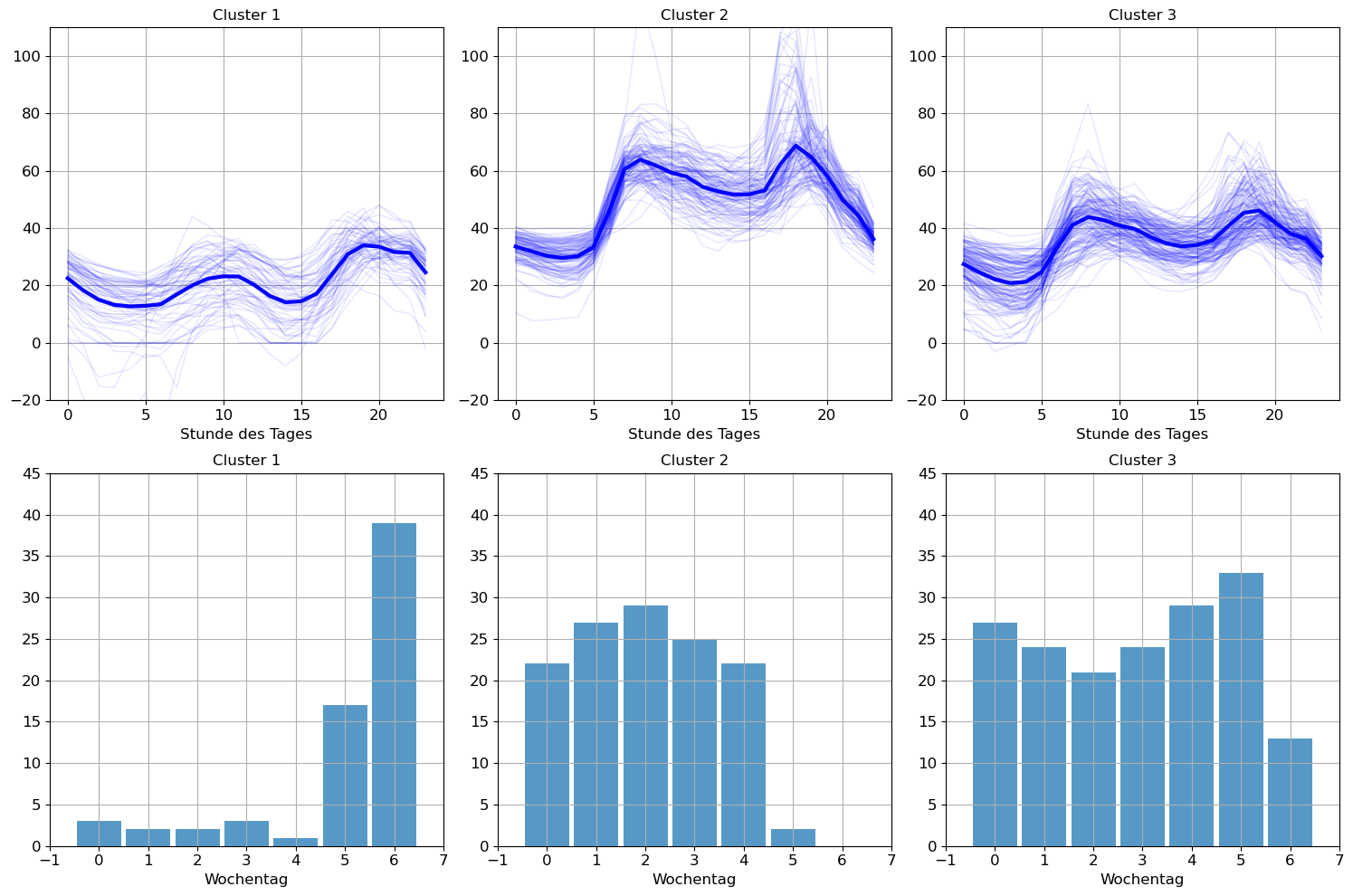
Grid Search mit Cross Validation
Aufgabe 3: Wirksamkeit von Werbung
Wir verwenden wieder den Datensatz von der Website zur ersten Ausgabe des Buches Introduction to Statistical Learning. Als Zielgröße nehmen wir wieder die Anzahl der Verkäufe (sales).
df = pd.read_csv('daten/Advertising.csv', index_col=0)
df.head(3)| TV | radio | newspaper | sales | |
|---|---|---|---|---|
| 1 | 230.1 | 37.8 | 69.2 | 22.1 |
| 2 | 44.5 | 39.3 | 45.1 | 10.4 |
| 3 | 17.2 | 45.9 | 69.3 | 9.3 |
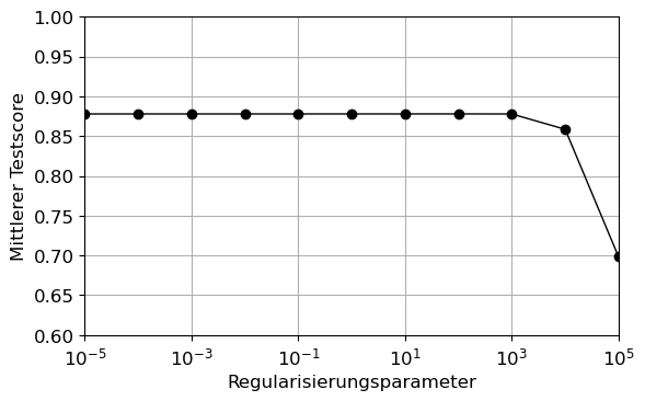
Verwenden Sie den Befehl GridSearchCV, um bei 10 Folds den besten alpha Wert aus \(10^{-5}, 10^{-4}, \ldots, 10^{4}, 10^{5}\) zu bestimmen und das finale Modell an Test-Datensatz zu evaluieren. Stellen Sie das Ergebnis grafisch dar.
Lösung:
from sklearn.model_selection import GridSearchCV

X = df.drop('sales', axis=1).values
y = df['sales'].values

param_grid = {'alpha': np.logspace(-5, 5, num=11)}

grid_search = GridSearchCV(Ridge(),
                           param_grid,
                           cv=10)

X_train, X_test, y_train, y_test = train_test_split(X, y, random_state=None)

grid_search.fit(X_train, y_train);

print(f"Test set score:  {grid_search.score(X_test, y_test):.2f}")
print(f"Best parameters: {grid_search.best_params_}")
print(f"Best estimator:  {grid_search.best_estimator_}")
print(f"Best cross-validation score: {grid_search.best_score_:.2f}")
Test set score: 0.90
Best parameters: {'alpha': 100.0}
Best estimator: Ridge(alpha=100.0)
Best cross-validation score: 0.88results = pd.DataFrame(grid_search.cv_results_)
results| mean_fit_time | std_fit_time | mean_score_time | std_score_time | param_alpha | params | split0_test_score | split1_test_score | split2_test_score | split3_test_score | split4_test_score | split5_test_score | split6_test_score | split7_test_score | split8_test_score | split9_test_score | mean_test_score | std_test_score | rank_test_score | |
|---|---|---|---|---|---|---|---|---|---|---|---|---|---|---|---|---|---|---|---|
| 0 | 0.000907 | 0.000619 | 0.000444 | 0.000157 | 0.00001 | {'alpha': 1e-05} | 0.910137 | 0.945325 | 0.832984 | 0.911533 | 0.777626 | 0.842344 | 0.921353 | 0.754907 | 0.931895 | 0.950119 | 0.877822 | 0.067231 | 8 |
| 1 | 0.000699 | 0.000176 | 0.000369 | 0.000090 | 0.0001 | {'alpha': 0.0001} | 0.910137 | 0.945325 | 0.832984 | 0.911533 | 0.777626 | 0.842344 | 0.921353 | 0.754907 | 0.931895 | 0.950119 | 0.877822 | 0.067231 | 7 |
| 2 | 0.000595 | 0.000030 | 0.000364 | 0.000073 | 0.001 | {'alpha': 0.001} | 0.910137 | 0.945325 | 0.832984 | 0.911533 | 0.777626 | 0.842344 | 0.921353 | 0.754907 | 0.931895 | 0.950119 | 0.877822 | 0.067231 | 6 |
| 3 | 0.000642 | 0.000050 | 0.000349 | 0.000029 | 0.01 | {'alpha': 0.01} | 0.910137 | 0.945325 | 0.832984 | 0.911533 | 0.777626 | 0.842344 | 0.921353 | 0.754907 | 0.931895 | 0.950119 | 0.877822 | 0.067231 | 5 |
| 4 | 0.000597 | 0.000061 | 0.000326 | 0.000019 | 0.1 | {'alpha': 0.1} | 0.910138 | 0.945325 | 0.832983 | 0.911533 | 0.777626 | 0.842344 | 0.921353 | 0.754907 | 0.931895 | 0.950119 | 0.877822 | 0.067231 | 4 |
| 5 | 0.000829 | 0.000211 | 0.000450 | 0.000126 | 1.0 | {'alpha': 1.0} | 0.910143 | 0.945327 | 0.832979 | 0.911535 | 0.777625 | 0.842347 | 0.921355 | 0.754907 | 0.931894 | 0.950117 | 0.877823 | 0.067231 | 3 |
| 6 | 0.001516 | 0.000616 | 0.000874 | 0.000456 | 10.0 | {'alpha': 10.0} | 0.910197 | 0.945342 | 0.832932 | 0.911551 | 0.777617 | 0.842368 | 0.921368 | 0.754907 | 0.931887 | 0.950092 | 0.877826 | 0.067237 | 2 |
| 7 | 0.000870 | 0.000101 | 0.000479 | 0.000048 | 100.0 | {'alpha': 100.0} | 0.910733 | 0.945487 | 0.832460 | 0.911709 | 0.777526 | 0.842576 | 0.921497 | 0.754907 | 0.931809 | 0.949846 | 0.877855 | 0.067296 | 1 |
| 8 | 0.000842 | 0.000125 | 0.000487 | 0.000096 | 1000.0 | {'alpha': 1000.0} | 0.915264 | 0.946655 | 0.827571 | 0.912980 | 0.776346 | 0.844030 | 0.922361 | 0.754593 | 0.930809 | 0.947152 | 0.877776 | 0.067915 | 9 |
| 9 | 0.001244 | 0.000537 | 0.000614 | 0.000191 | 10000.0 | {'alpha': 10000.0} | 0.915528 | 0.941809 | 0.774240 | 0.909163 | 0.751600 | 0.827129 | 0.908776 | 0.736587 | 0.909373 | 0.910491 | 0.858470 | 0.074130 | 10 |
| 10 | 0.000651 | 0.000151 | 0.000378 | 0.000077 | 100000.0 | {'alpha': 100000.0} | 0.728213 | 0.810014 | 0.547481 | 0.823363 | 0.591371 | 0.648632 | 0.756350 | 0.621330 | 0.743686 | 0.711976 | 0.698241 | 0.087866 | 11 |
plt.figure()
plt.plot(param_grid['alpha'], results.mean_test_score, 'o-',c='black')
plt.xticks(param_grid['alpha'])
plt.ylim(0.6,1)
plt.xlim(1e-5,1e5)
plt.xlabel('Regularisierungsparameter')
plt.ylabel('Mittlerer Testscore')
plt.xscale('log')
plt.grid(True)