import pandas as pd
import matplotlib.pyplot as plt
import numpy as np
import mglearnModel Evaluation
Book
This IPython notebook follows the book Introduction to Machine Learning with Python by Andreas Mueller and Sarah Guido and uses material from its github repository and from the working files of the training course Advanced Machine Learning with scikit-learn. Excerpts taken from the book are displayed in italic letters.
The contents of this Jupyter notebook corresponds in the book Introduction to Machine Learning with Python to:
- Chapter 5 “Model Evaluation and Improvement”: p. 251 to 270
Python
# import matplotlib.cbook
# import warnings
# warnings.filterwarnings("ignore",category=matplotlib.cbook.mplDeprecation)
Introduction
Typical Procedure So Far: Example
from sklearn.datasets import make_blobs
from sklearn.linear_model import LogisticRegression
from sklearn.model_selection import train_test_split

# create a synthetic dataset
X, y = make_blobs(random_state=0)

# split data and labels into a training and a test set
X_train, X_test, y_train, y_test = train_test_split(X, y, random_state=0)

# Instantiate a model and fit it to the training set
logreg = LogisticRegression(solver='lbfgs', multi_class='auto').fit(X_train, y_train)

# evaluate the model on the test set
print(f"Test set score: {logreg.score(X_test, y_test):.2f}")
Test set score: 0.88Monte Carlo Simulation
Statistik des Test set scores über viele Train-Testdatensplits
runs = 500
lr = LogisticRegression(solver='lbfgs', multi_class='auto')
my_scores = []

for k in range(runs):
    X_train, X_test, y_train, y_test = train_test_split(X, y)
    my_scores.append(lr.fit(X_train, y_train).score(X_test, y_test))

plt.figure(figsize=(6,4))
plt.hist(my_scores, bins = 7)
plt.xlabel("test set scores")
plt.grid(True)
print(f"Mean test set score   : {np.mean(my_scores):.2f}")
print(f"Std. of test set score: {np.std( my_scores):.2f}")
Mean test set score : 0.90
Std. of test set score: 0.06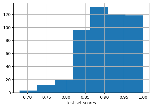
Cross-validation
Method
mglearn.plots.plot_cross_validation()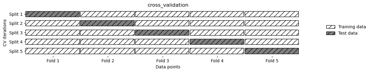
Cross-validation in scikit-learn
from sklearn.datasets        import load_iris
from sklearn.linear_model    import LogisticRegression
from sklearn.model_selection import cross_val_score

iris = load_iris()
logreg = LogisticRegression(solver='liblinear', multi_class='auto')

scores = cross_val_score(logreg, iris.data, iris.target, cv=5)
print(f"Cross validation test scores: {scores}")
Cross validation test scores: [1. 0.96666667 0.93333333 0.9 1. ]print(f"Average of cross-validation test score: {scores.mean():.2f}")
print(f"St.dev. of cross-validation test score: {scores.std():.2f}")Average of cross-validation test score: 0.96
St.dev. of cross-validation test score: 0.04Benefits of Cross-Validation
- less randomization effects
- Each sample will be in the testing set exactly once.
- Having multiple splits of the data also provides some information about how sensitive the model is to the selection of the training dataset: average and standard deviation of cross-validation scores
- When using for example 10-fold cross-validation, we use nine-tenths of the data (90%) to fit the model. More data will usually result in more accurate models.
Warnings:
- increased computational cost
- Cross-validation is not a way to build a model that can be applied to new data. Cross-validation does not return a model.
Stratified K-Fold cross-validation and other strategies
from sklearn.datasets import load_iris
iris = load_iris()
print(f"Iris labels:\n{iris.target}")
Iris labels:
[0 0 0 0 0 0 0 0 0 0 0 0 0 0 0 0 0 0 0 0 0 0 0 0 0 0 0 0 0 0 0 0 0 0 0 0 0
0 0 0 0 0 0 0 0 0 0 0 0 0 1 1 1 1 1 1 1 1 1 1 1 1 1 1 1 1 1 1 1 1 1 1 1 1
1 1 1 1 1 1 1 1 1 1 1 1 1 1 1 1 1 1 1 1 1 1 1 1 1 1 2 2 2 2 2 2 2 2 2 2 2
2 2 2 2 2 2 2 2 2 2 2 2 2 2 2 2 2 2 2 2 2 2 2 2 2 2 2 2 2 2 2 2 2 2 2 2 2
2 2]As the simple k-fold strategy fails here, scikit-learn does not use it for classification, but rather uses stratified k-fold cross-validation. In stratified cross-validation, we split the data such that the proportions between classes are the same in each fold as they are in the whole dataset.
mglearn.plots.plot_stratified_cross_validation()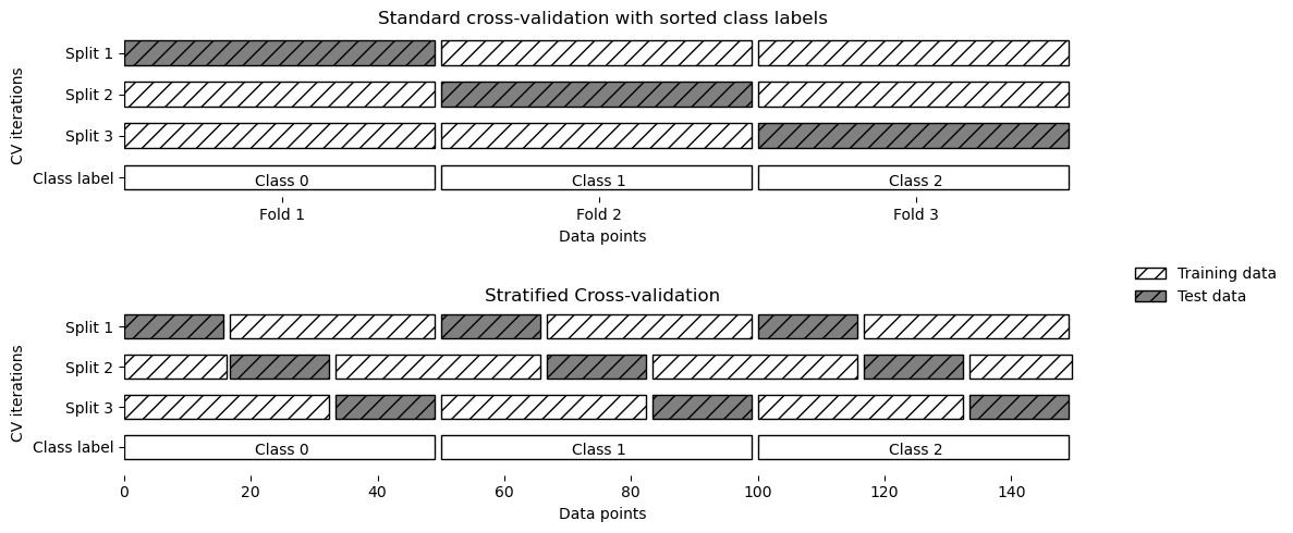
For regression, scikit-learn uses the standard k-fold cross-validation by default.
More control over cross-validation
No Stratification
from sklearn.model_selection import KFold

kfold = KFold(n_splits=3)
print(f"Cross-validation scores:\n{cross_val_score(logreg, iris.data, iris.target, cv=kfold)}")
Cross-validation scores:
[0. 0. 0.]cross_val_score(logreg, iris.data, iris.target, cv=3)array([0.96, 0.96, 0.94])Explicit Stratification
from sklearn.model_selection import StratifiedKFold

skfold = StratifiedKFold(n_splits=3)
print(f"Cross-validation scores:\n{cross_val_score(logreg, iris.data, iris.target, cv=skfold)}")
Cross-validation scores:
[0.96 0.96 0.94]Shuffling Data
Instead of stratifying the folds one can shuffle the data to remove the ordering of the samples by label.
kfold = KFold(n_splits=5, shuffle=True, random_state=0)

print(f"Cross-validation scores:\n{cross_val_score(logreg, iris.data, iris.target, cv=kfold)}")
Cross-validation scores:
[0.96666667 0.9 0.96666667 0.96666667 0.93333333]Leave-One-Out cross-validation
from sklearn.model_selection import LeaveOneOut

loo = LeaveOneOut()
scores = cross_val_score(logreg, iris.data, iris.target, cv=loo)
print(f"Number of cv iterations: {len(scores)}")
print(f"Mean accuracy: {scores.mean():.2f}")
Number of cv iterations: 150
Mean accuracy: 0.95Shuffle-Split cross-validation
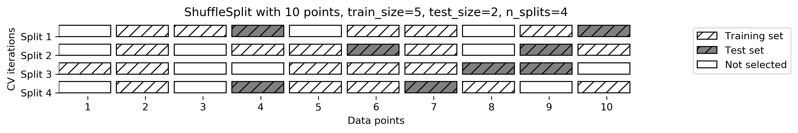
You can use integers for train_size and test_size to use absolute sizes for these sets, or floating-point numbers to use fractions of the whole dataset.
from sklearn.model_selection import ShuffleSplit

shuffle_split = ShuffleSplit(test_size=.5, train_size=.5, n_splits=10, random_state=0)
scores = cross_val_score(logreg, iris.data, iris.target, cv=shuffle_split)
print(f"Cross-validation scores:\n{scores}")
Cross-validation scores:
[0.84 0.93333333 0.90666667 1. 0.90666667 0.93333333
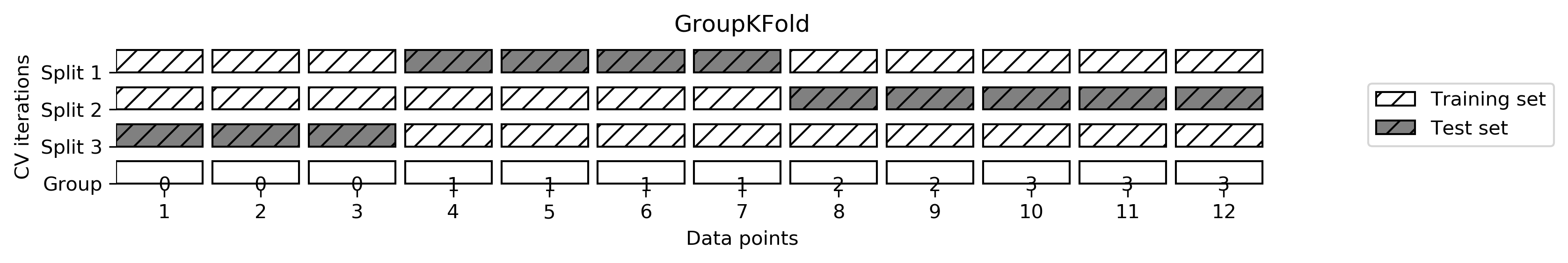
0.94666667 1. 0.90666667 0.88 ]Cross-validation with groups
For example in medical applications, to have groups in the data is very common. You might have multiple samples from the same patient, but are interested in generalizing to new patients. Similarly, in speech recognition, you might have multiple recordings of the same speaker in your dataset, but are interested in recognizing speech of new speakers.
from sklearn.model_selection import GroupKFold

# create synthetic dataset
X, y = make_blobs(n_samples=12, random_state=0)

# assume the first three samples belong to the same group,
# then the next four etc.
groups = [0, 0, 0, 1, 1, 1, 1, 2, 2, 3, 3, 3]

print(f'target values:    {y}')
print(f'group membership: {groups}')
target values: [1 0 2 0 0 1 1 2 0 2 2 1]
group membership: [0, 0, 0, 1, 1, 1, 1, 2, 2, 3, 3, 3]scores = cross_val_score(logreg, X, y, groups=groups, cv=GroupKFold(n_splits=3))
print(f"Cross-validation scores:\n{scores}")Cross-validation scores:
[0.75 0.8 0.66666667]Grid Search
find best model by evaluating different model parameters
Simple Grid-Search
from sklearn.datasets import load_breast_cancer

cancer = load_breast_cancer()
X_train, X_test, y_train, y_test = train_test_split(
    cancer.data, cancer.target, stratify=cancer.target, random_state=110)

from sklearn.neighbors import KNeighborsClassifier

best_score = 0
for k in [1, 2, 3, 4, 5, 6, 7, 8, 9, 10]:
    clf = KNeighborsClassifier(n_neighbors=k)
    clf.fit(X_train, y_train)
    # evaluate the kNN on the test set
    score = clf.score(X_test, y_test)
    # if we got a better score, store the score and parameters
    if score > best_score:
        best_score = score
        best_parameter = k

print(f"Best score: {best_score:.2f}")
print(f"Best k    : {best_parameter}")
Best score: 0.94
Best k : 6We tried many different parameters and selected the one with best accuracy on the test set, but this accuracy won’t necessarily carry over to new data. Because we used the test data to adjust the parameters, we can no longer use it to assess how good the model is. This is the same reason we needed to split the data into training and test sets in the first place; we need an independent dataset to evaluate, one that was not used to create the model.
The danger of overfitting the parameters and the validation set

# split data into train+validation set and test set
X_trainval, X_test, y_trainval, y_test = train_test_split(
    cancer.data, cancer.target, stratify=cancer.target, random_state=110)

# split train+validation set into training and validation set
X_train, X_valid, y_train, y_valid = train_test_split(
    X_trainval, y_trainval, random_state=1)

print(f"Size of training set: {X_train.shape[0]}\n\
Size of validation set: {X_valid.shape[0]}\n\
Size of test set: {X_test.shape[0]}")
Size of training set: 319
Size of validation set: 107
Size of test set: 143best_score = 0
for k in [1, 2, 3, 4, 5, 6, 7, 8, 9, 10]:
clf = KNeighborsClassifier(n_neighbors=k)
clf.fit(X_train, y_train)
# evaluate the kNN on the test set
score = clf.score(X_valid, y_valid)
# if we got a better score, store the score and parameters
if score > best_score:
best_score = score
best_parameter = k
# rebuild a model on the combined training and validation set,
# and evaluate it on the test set
clf = KNeighborsClassifier(n_neighbors=best_parameter)
clf.fit(X_trainval, y_trainval)
test_score = clf.score(X_test, y_test)
print(f"Best score on validation set: {best_score:.2f}")
print(f"Best parameter: {best_parameter}")
print(f"Test set score with best parameter: {test_score:.2f}")Best score on validation set: 0.92
Best parameter: 6
Test set score with best parameter: 0.94Grid-search with cross-validation
(A) Manual Grid Search:
# manual_grid_search_cv
best_score = 0
for k in [1, 2, 3, 4, 5, 6, 7, 8, 9, 10]:
    clf = KNeighborsClassifier(n_neighbors=k)
    # perform cross-validation
    scores = cross_val_score(clf, X_trainval, y_trainval, cv=5)
    # compute mean cross-validation accuracy
    score = np.mean(scores)
    # if we got a better score, store the score and parameters
    if score > best_score:
        best_score = score
        best_parameter = k

# rebuild a model on the combined training and validation set
# and evaluate it on the test set
clf = KNeighborsClassifier(n_neighbors=best_parameter)
clf.fit(X_trainval, y_trainval)
test_score = clf.score(X_test, y_test)
print(f"Best score on validation set: {best_score:.2f}")
print(f"Best parameter: {best_parameter}")
print(f"Test set score with best parameter: {test_score:.2f}")
Best score on validation set: 0.94
Best parameter: 9
Test set score with best parameter: 0.92mglearn.plots.plot_grid_search_overview()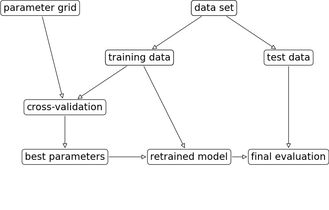
(B) Grid Search Using GridSearchCV:
Because grid search with cross-validation is such a commonly used method to adjust parameters, scikit-learn provides the GridSearchCV class.
param_grid = {'n_neighbors': [1, 2, 3, 4, 5, 6, 7, 8, 9, 10, 11, 12, 13, 14, 15, 16, 17, 18, 19, 20]}
print(f"Parameter grid:\n{param_grid}")
Parameter grid:
{'n_neighbors': [1, 2, 3, 4, 5, 6, 7, 8, 9, 10, 11, 12, 13, 14, 15, 16, 17, 18, 19, 20]}from sklearn.model_selection import GridSearchCV
from sklearn.neighbors import KNeighborsClassifier
grid_search = GridSearchCV(KNeighborsClassifier(),
param_grid,
cv=5,
return_train_score=True)
X_train, X_test, y_train, y_test = train_test_split(
cancer.data, cancer.target, stratify=cancer.target, random_state=110)
grid_search.fit(X_train, y_train)GridSearchCV(cv=5, estimator=KNeighborsClassifier(),
param_grid={'n_neighbors': [1, 2, 3, 4, 5, 6, 7, 8, 9, 10, 11, 12,
13, 14, 15, 16, 17, 18, 19, 20]},
return_train_score=True)In a Jupyter environment, please rerun this cell to show the HTML representation or trust the notebook. On GitHub, the HTML representation is unable to render, please try loading this page with nbviewer.org.
GridSearchCV(cv=5, estimator=KNeighborsClassifier(),
             param_grid={'n_neighbors': [1, 2, 3, 4, 5, 6, 7, 8, 9, 10, 11, 12,
                                         13, 14, 15, 16, 17, 18, 19, 20]},
return_train_score=True)KNeighborsClassifier()
KNeighborsClassifier()
print(f"Test set score: {grid_search.score(X_test, y_test):.2f}")
print(f"Best parameters: {grid_search.best_params_}")
print(f"Best cross-validation score: {grid_search.best_score_:.2f}")
Test set score: 0.90
Best parameters: {'n_neighbors': 12}
Best cross-validation score: 0.94print(f"Best estimator:\n{grid_search.best_estimator_}")Best estimator:
KNeighborsClassifier(n_neighbors=12)Analyzing the result of cross-validation
# convert to Dataframe
import pandas as pd
results = pd.DataFrame(grid_search.cv_results_)

results| mean_fit_time | std_fit_time | mean_score_time | std_score_time | param_n_neighbors | params | split0_test_score | split1_test_score | split2_test_score | split3_test_score | ... | mean_test_score | std_test_score | rank_test_score | split0_train_score | split1_train_score | split2_train_score | split3_train_score | split4_train_score | mean_train_score | std_train_score | |
|---|---|---|---|---|---|---|---|---|---|---|---|---|---|---|---|---|---|---|---|---|---|
| 0 | 0.000669 | 0.000314 | 0.008900 | 0.012498 | 1 | {'n_neighbors': 1} | 0.872093 | 0.905882 | 0.941176 | 0.952941 | ... | 0.910889 | 0.031718 | 19 | 1.000000 | 1.000000 | 1.000000 | 1.000000 | 1.000000 | 1.000000 | 0.000000 |
| 1 | 0.000428 | 0.000054 | 0.002953 | 0.000355 | 2 | {'n_neighbors': 2} | 0.872093 | 0.870588 | 0.894118 | 0.929412 | ... | 0.894419 | 0.022011 | 20 | 0.973529 | 0.967742 | 0.961877 | 0.961877 | 0.967742 | 0.966553 | 0.004364 |
| 2 | 0.000397 | 0.000010 | 0.002671 | 0.000116 | 3 | {'n_neighbors': 3} | 0.895349 | 0.929412 | 0.929412 | 0.964706 | ... | 0.932011 | 0.022408 | 16 | 0.958824 | 0.941349 | 0.953079 | 0.932551 | 0.947214 | 0.946603 | 0.009129 |
| 3 | 0.000388 | 0.000012 | 0.002594 | 0.000053 | 4 | {'n_neighbors': 4} | 0.906977 | 0.917647 | 0.929412 | 0.964706 | ... | 0.931984 | 0.019964 | 18 | 0.955882 | 0.947214 | 0.950147 | 0.935484 | 0.950147 | 0.947775 | 0.006758 |
| 4 | 0.000401 | 0.000026 | 0.002656 | 0.000060 | 5 | {'n_neighbors': 5} | 0.895349 | 0.941176 | 0.952941 | 0.952941 | ... | 0.936717 | 0.021343 | 6 | 0.952941 | 0.953079 | 0.950147 | 0.932551 | 0.938416 | 0.945427 | 0.008393 |
| 5 | 0.000390 | 0.000027 | 0.002693 | 0.000090 | 6 | {'n_neighbors': 6} | 0.895349 | 0.941176 | 0.929412 | 0.964706 | ... | 0.932011 | 0.022408 | 16 | 0.952941 | 0.953079 | 0.950147 | 0.932551 | 0.944282 | 0.946600 | 0.007714 |
| 6 | 0.000390 | 0.000013 | 0.002720 | 0.000106 | 7 | {'n_neighbors': 7} | 0.895349 | 0.941176 | 0.952941 | 0.964706 | ... | 0.936717 | 0.023796 | 6 | 0.952941 | 0.941349 | 0.941349 | 0.935484 | 0.938416 | 0.941908 | 0.005930 |
| 7 | 0.000396 | 0.000016 | 0.002720 | 0.000119 | 8 | {'n_neighbors': 8} | 0.895349 | 0.941176 | 0.952941 | 0.964706 | ... | 0.936717 | 0.023796 | 6 | 0.952941 | 0.947214 | 0.938416 | 0.935484 | 0.938416 | 0.942494 | 0.006539 |
| 8 | 0.000398 | 0.000018 | 0.002710 | 0.000066 | 9 | {'n_neighbors': 9} | 0.895349 | 0.941176 | 0.964706 | 0.952941 | ... | 0.939070 | 0.023537 | 3 | 0.950000 | 0.941349 | 0.929619 | 0.935484 | 0.935484 | 0.938387 | 0.006890 |
| 9 | 0.000393 | 0.000014 | 0.002713 | 0.000060 | 10 | {'n_neighbors': 10} | 0.895349 | 0.941176 | 0.964706 | 0.964706 | ... | 0.939070 | 0.025782 | 3 | 0.950000 | 0.944282 | 0.938416 | 0.932551 | 0.938416 | 0.940733 | 0.005935 |
| 10 | 0.000402 | 0.000016 | 0.002763 | 0.000055 | 11 | {'n_neighbors': 11} | 0.895349 | 0.941176 | 0.964706 | 0.952941 | ... | 0.936717 | 0.023796 | 6 | 0.950000 | 0.941349 | 0.935484 | 0.932551 | 0.938416 | 0.939560 | 0.005987 |
| 11 | 0.000406 | 0.000023 | 0.002763 | 0.000072 | 12 | {'n_neighbors': 12} | 0.895349 | 0.941176 | 0.964706 | 0.964706 | ... | 0.941423 | 0.025326 | 1 | 0.950000 | 0.944282 | 0.932551 | 0.932551 | 0.941349 | 0.940147 | 0.006797 |
| 12 | 0.000396 | 0.000020 | 0.002754 | 0.000105 | 13 | {'n_neighbors': 13} | 0.895349 | 0.929412 | 0.964706 | 0.964706 | ... | 0.936717 | 0.026019 | 6 | 0.950000 | 0.941349 | 0.932551 | 0.932551 | 0.938416 | 0.938974 | 0.006481 |
| 13 | 0.000425 | 0.000014 | 0.002842 | 0.000082 | 14 | {'n_neighbors': 14} | 0.895349 | 0.941176 | 0.964706 | 0.964706 | ... | 0.941423 | 0.025326 | 1 | 0.950000 | 0.941349 | 0.929619 | 0.932551 | 0.938416 | 0.938387 | 0.007135 |
| 14 | 0.000402 | 0.000022 | 0.002937 | 0.000254 | 15 | {'n_neighbors': 15} | 0.883721 | 0.929412 | 0.964706 | 0.964706 | ... | 0.934391 | 0.029850 | 11 | 0.947059 | 0.941349 | 0.935484 | 0.932551 | 0.941349 | 0.939558 | 0.005067 |
| 15 | 0.000398 | 0.000020 | 0.002843 | 0.000108 | 16 | {'n_neighbors': 16} | 0.883721 | 0.941176 | 0.964706 | 0.964706 | ... | 0.936744 | 0.029828 | 5 | 0.947059 | 0.941349 | 0.932551 | 0.935484 | 0.938416 | 0.938972 | 0.004995 |
| 16 | 0.000492 | 0.000119 | 0.003743 | 0.001573 | 17 | {'n_neighbors': 17} | 0.883721 | 0.929412 | 0.964706 | 0.952941 | ... | 0.932038 | 0.027758 | 13 | 0.941176 | 0.941349 | 0.932551 | 0.932551 | 0.935484 | 0.936622 | 0.003938 |
| 17 | 0.000413 | 0.000012 | 0.003096 | 0.000478 | 18 | {'n_neighbors': 18} | 0.883721 | 0.929412 | 0.964706 | 0.952941 | ... | 0.932038 | 0.027758 | 13 | 0.941176 | 0.941349 | 0.932551 | 0.932551 | 0.938416 | 0.937209 | 0.003943 |
| 18 | 0.000414 | 0.000010 | 0.003097 | 0.000301 | 19 | {'n_neighbors': 19} | 0.883721 | 0.929412 | 0.964706 | 0.952941 | ... | 0.934391 | 0.027933 | 11 | 0.941176 | 0.938416 | 0.929619 | 0.932551 | 0.932551 | 0.934863 | 0.004259 |
| 19 | 0.000423 | 0.000031 | 0.003011 | 0.000155 | 20 | {'n_neighbors': 20} | 0.883721 | 0.929412 | 0.964706 | 0.952941 | ... | 0.932038 | 0.027758 | 13 | 0.941176 | 0.944282 | 0.932551 | 0.932551 | 0.935484 | 0.937209 | 0.004736 |
20 rows × 21 columns
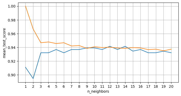
plt.figure(figsize=(8, 4))
plt.plot(param_grid['n_neighbors'], results.mean_test_score)
plt.plot(param_grid['n_neighbors'], results.mean_train_score)
plt.xticks(param_grid['n_neighbors'])
plt.xlabel('n_neighbors')
plt.ylabel('mean_test_score')
plt.grid(True)