import pandas as pd
import matplotlib.pyplot as plt
import numpy as np
import mglearn
from IPython.display import ImageSupervised Learning 2
Book
This IPython notebook follows the book Introduction to Machine Learning with Python by Andreas Mueller and Sarah Guido and uses material from its github repository and from the working files of the training course Advanced Machine Learning with scikit-learn. Excerpts taken from the book are displayed in italic letters.
The contents of this Jupyter notebook corresponds in the book Introduction to Machine Learning with Python to:
- Chapter 2 “Supervised Learning”: p. 44 to 92
Python
if 0:
    import warnings
    warnings.filterwarnings("ignore")
Linear Models for Regression
Overview
Examples:
some energy-related articles using regression:
- Using regression analysis to predict the future energy consumption of a supermarket in the UK
- Multiple regression models for energy consumption of office buildings in different climates in China
- Multiple regression models to predict the annual energy consumption in the Spanish banking sector
Goals:
- find relationships between quantities described with a formula
- find the strengths, directions and significances of the relationships
Procedure:
- visual inspection of data, maybe transform or select data parts
- fit different regression models to data
- choose best model(s) using cross validation or/and p-values
- make predictions or simulations from the fitted model(s)
Models:
- Linear Regression aka Ordinary Least Squares
- Ridge Regression
- Lasso
Linear Regression aka Ordinary Least Squares
Eine lineare Regression liefert die optimalen Koeffizienten \(c_k\) der Formel
\[\hat{y} = c_0 + c_1 x_1 + \ldots + c_m x_m\]
durch Minimierung des mittleren quadratischen Fehlers zwischen Target \(y\) und Fit \(\hat{y}\) auf den Trainingsdaten:
\[\text{min. }\sum_{i=1}^n (y_i - c_0 - \sum_{k=1}^m x_{ik} c_k)^2.\]
- Kurzschreibweise: \(y \sim x_1 + \ldots + x_m\)
- Das Modell verwendet die \(m\) Features (=Regressoren) \(x_1\) bis \(x_m\).
- Der konstante Offset \(c_0\) heißt im Englischen intercept.
- \(\hat{y}\) bezeichnet den Fit bzw. die Prognose des Targets aus den Features.
- Der Fit/Prognose-Fehler ist die Differenz \(y - \hat{y}\) von Target zu Fit/Prognose.
- Spezialfall für ein Feature: \(y \sim x_1\) bzw. \(\hat{y} = c_0 + c_1 x_1\)
- Anzahl Trainingsdaten > Anzahl Features, sonst starkes Overfitting!
# Grafische Darstellung für Y ~ X:

mglearn.plots.plot_linear_regression_wave()
w[0]: 0.393906 b: -0.031804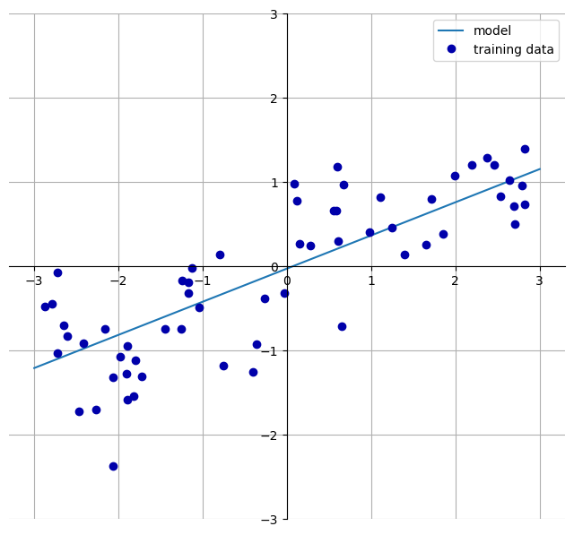
Implementierung am Beispiel des wave Datensatzes:
from sklearn.model_selection import train_test_split
from sklearn.linear_model    import LinearRegression

X, y = mglearn.datasets.make_wave(n_samples=60)
X_train, X_test, y_train, y_test = train_test_split(X, y, random_state=42)

lr = LinearRegression().fit(X_train, y_train)print(f"lr.coef_: {lr.coef_}")
print(f"lr.intercept_: {lr.intercept_}")lr.coef_: [0.39390555]
lr.intercept_: -0.031804343026759746print(f"Training set score: {lr.score(X_train, y_train):.2f}")
print(f"Test set score: {lr.score(X_test, y_test):.2f}")Training set score: 0.67
Test set score: 0.66Regularization with Ridge Regression
Die optimalen Ridge-Koeffizienten \(c_j\) minimieren für einen vorgegebenen \(\alpha\)-Wert die Zielfunktion
\[\text{min. }\sum_{i=1}^n (y_i - c_0 - \sum_{k=1}^m x_{ik} c_k)^2 + \alpha \sum_{k=1} c_k^2.\]
from sklearn.linear_model import Ridge

# X, y = mglearn.datasets.load_extended_boston()
data_url = "http://lib.stat.cmu.edu/datasets/boston"
raw_df = pd.read_csv(data_url, sep="\s+", skiprows=22, header=None)
X = np.hstack([raw_df.values[::2, :], raw_df.values[1::2, :2]])
y = raw_df.values[1::2, 2]

X_train, X_test, y_train, y_test = train_test_split(X, y, random_state=0)

ridge = Ridge().fit(X_train, y_train)   # default alpha=1.0

print(f"Training set score: {ridge.score(X_train, y_train):.2f}")
print(f"Test     set score: {ridge.score(X_test, y_test):.2f}")
Training set score: 0.77
Test set score: 0.63plt.figure(figsize=(8, 5))
plt.stem(np.concatenate(([ridge.intercept_], ridge.coef_)))
# plt.ylim(-20, 20)
plt.xlabel('feature')
plt.ylabel('ridge regression coefficient')
plt.grid(True)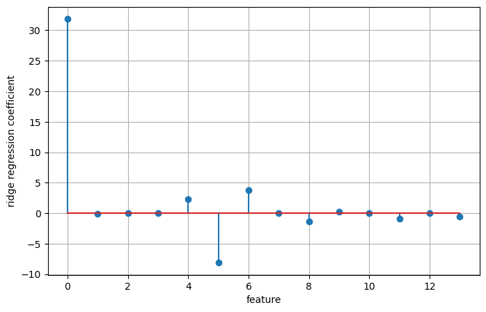
ridge10 = Ridge(alpha=10).fit(X_train, y_train)

print(f"Training set score: {ridge10.score(X_train, y_train):.2f}")
print(f"Test set score: {ridge10.score(X_test, y_test):.2f}")
Training set score: 0.76
Test set score: 0.61ridge01 = Ridge(alpha=0.1).fit(X_train, y_train)
print(f"Training set score: {ridge01.score(X_train, y_train):.2f}")
print(f"Test set score: {ridge01.score(X_test, y_test):.2f}")Training set score: 0.77
Test set score: 0.63Lernkurve:
Another way to understand the influence of regularization is to fix a value of alpha but vary the amount of training data available. In the following figure, we subsample the Boston Housing dataset and evaluate Linear Regression and Ridge(alpha=1) on subsets of increasing size. Plots that show model performance as a function of dataset size are called learning curves.
plt.figure(figsize=(8, 6))
mglearn.plots.plot_ridge_n_samples()
plt.grid(True)
The lesson here is that with enough training data, regularization becomes less important.
Regularization with Lasso Regression
Die optimalen Ridge-Koeffizienten \(c_j\) minimieren für einen vorgegebenen \(\alpha\)-Wert die Zielfunktion
\[\text{min. }\frac{1}{2n}\sum_{i=1}^n (y_i - c_0 - \sum_{k=1}^m x_{ik} c_k)^2 + \alpha \sum_{k=1} |c_k|.\]
As a consequence, some coefficients are exactly zero. This means some features are entirely ignored by the model. This can be seen as a form of automatic feature selection. Having some coefficients be exactly zero often makes a model easier to interpret, and can reveal the most important features of your model.
from sklearn.linear_model import Lasso

lasso = Lasso().fit(X_train, y_train)  # default alpha = 1

print(f"Training set score: {lasso.score(X_train, y_train):.2f}")
print(f"Test     set score: {lasso.score(X_test, y_test):.2f}")
print(f"Number of features used: {np.sum(lasso.coef_ != 0)}")

plt.figure(figsize=(8, 5))
plt.stem(np.concatenate(([lasso.intercept_], lasso.coef_)))
plt.xlabel('feature')
plt.ylabel('lasso regression coefficient')
plt.grid(True)
Training set score: 0.72
Test set score: 0.55
Number of features used: 11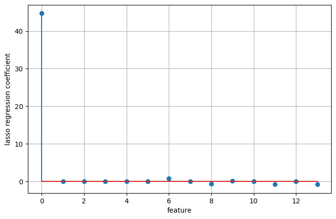
# we increase the default setting of "max_iter",
# otherwise the model would warn us that we should increase max_iter.

lasso001 = Lasso(alpha=0.01, max_iter=100000).fit(X_train, y_train)

print(f"Training set score: {lasso001.score(X_train, y_train):.2f}")
print(f"Test set score: {lasso001.score(X_test, y_test):.2f}")
print(f"Number of features used: {np.sum(lasso001.coef_ != 0)}")

plt.figure(figsize=(8, 5))
plt.stem(np.concatenate(([lasso001.intercept_], lasso001.coef_)))
plt.xlabel('feature')
plt.ylabel('lasso001 regression coefficient')
plt.grid(True)
Training set score: 0.77
Test set score: 0.63
Number of features used: 13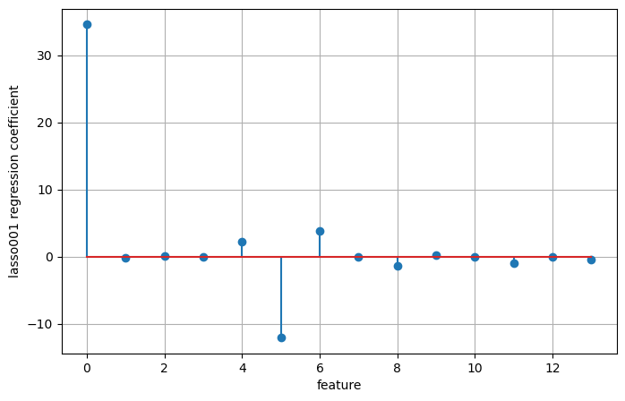
lasso00001 = Lasso(alpha=0.0001, max_iter=100000).fit(X_train, y_train)

print(f"Training set score: {lasso00001.score(X_train, y_train):.2f}")
print(f"Test     set score: {lasso00001.score(X_test, y_test):.2f}")
print(f"Number of features used: {np.sum(lasso00001.coef_ != 0)}")
Training set score: 0.77
Test set score: 0.64
Number of features used: 13Linear Models for Classification
Binary Linear Classification Models
- Falls \(\hat{y} = c_0 + c_1 x_1 + \ldots + c_m x_m >0\) ist, wird Klasse +1 vorhergesagt.
- Falls \(\hat{y} = c_0 + c_1 x_1 + \ldots + c_m x_m <0\) ist, wird Klasse -1 vorhergesagt.
Die Entscheidungsgrenze ist linear, d. h. eine Gerade, Ebene oder Hyperbene.
Die Algorithmen unterscheiden sich in
- der Methode, wie die Koeffizienten \(c_k\) aus den Trainingsdaten berechnet werden.
- der Art, wie Regularisierung implementiert ist.
Die zwei üblichsten Algorithmen sind:
Beide Algorithmen verwenden standardmäßig eine L2-Regularisierung, vgl. Ridge-Regression. Achtung: Je größer der Regularisierungsparamter \(C\) ist, umso geringer die Regularisierung - also gerade umgekehrt zum Paramter \(\alpha\) bei Ridge-Regression und Lasso. Eine L1-Regularisierung ist auch auswählbar und führt wiederum zu Modellen mit wenigen Koeffizienten.
from sklearn.linear_model import LogisticRegression
from sklearn.svm          import LinearSVC

from sklearn.model_selection import train_test_split
Beispiel: Synthetische Daten
X, y = mglearn.datasets.make_forge()

clf = LogisticRegression().fit(X, y)

mglearn.plots.plot_2d_separator(clf, X, fill=False, eps=0.5, alpha=.7)
mglearn.discrete_scatter(X[:, 0], X[:, 1], y)
plt.title("LogisticRegression")
plt.xlabel("Feature 0")
plt.ylabel("Feature 1");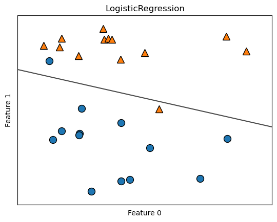
clf = LinearSVC(max_iter=5000).fit(X, y)
mglearn.plots.plot_2d_separator(clf, X, fill=False, eps=0.5, alpha=.7)
mglearn.discrete_scatter(X[:, 0], X[:, 1], y)
plt.title("LinearSVC")
plt.xlabel("Feature 0")
plt.ylabel("Feature 1");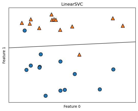
mglearn.plots.plot_linear_svc_regularization()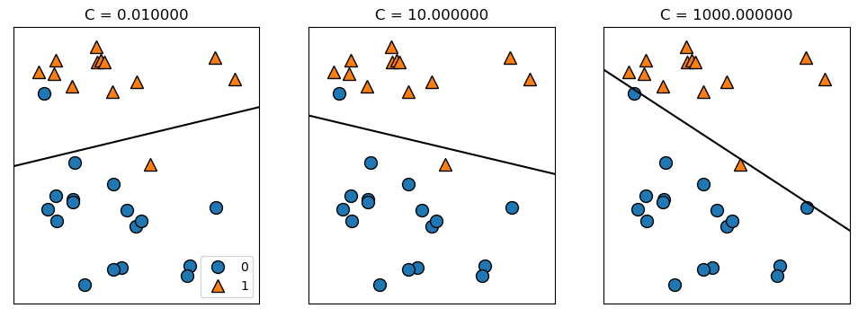
Beispiel: Brustkrebsdaten mit Logistischer Regression
from sklearn.datasets import load_breast_cancer
cancer = load_breast_cancer()

X_train, X_test, y_train, y_test = train_test_split(
    cancer.data, cancer.target, stratify=cancer.target, random_state=42)

logreg = LogisticRegression(max_iter=5000).fit(X_train, y_train)  # default: C=1

print(f"Training set score: {logreg.score(X_train, y_train):.3f}")
print(f"Test     set score: {logreg.score(X_test, y_test):.3f}")
Training set score: 0.958
Test set score: 0.958logreg100 = LogisticRegression(max_iter=5000, C=100).fit(X_train, y_train)
print(f"Training set score: {logreg100.score(X_train, y_train):.3f}")
print(f"Test set score: {logreg100.score(X_test, y_test):.3f}")Training set score: 0.981
Test set score: 0.965logreg001 = LogisticRegression(max_iter=5000, C=0.01).fit(X_train, y_train)
print(f"Training set score: {logreg001.score(X_train, y_train):.3f}")
print(f"Test set score: {logreg001.score(X_test, y_test):.3f}")Training set score: 0.953
Test set score: 0.951plt.figure(figsize=(10, 7))
plt.plot(logreg100.coef_.T, '^', label="C=100")
plt.plot(logreg.coef_.T, 'o', label="C=1")
plt.plot(logreg001.coef_.T, 'v', label="C=0.001")
plt.xticks(range(cancer.data.shape[1]), cancer.feature_names, rotation=90)
plt.hlines(0, 0, cancer.data.shape[1])
plt.ylim(-5, 5)
plt.xlabel("Coefficient index")
plt.ylabel("Coefficient magnitude")
plt.legend()
plt.grid(True)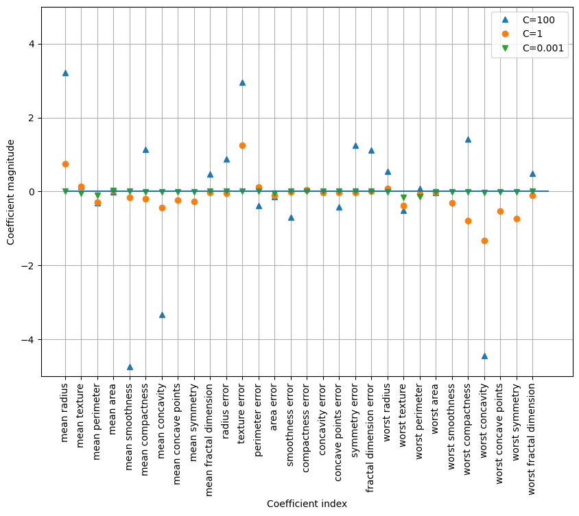
plt.figure(figsize=(10, 7))
for C, marker in zip([0.001, 1, 100], ['o', '^', 'v']):
    lr_l1 = LogisticRegression(max_iter=5000, solver='liblinear', C=C, penalty="l1").fit(X_train, y_train)
    print(f"Training accuracy of l1 logreg with C={C:.3f}: {lr_l1.score(X_train, y_train):.2f}")
    print(f"Test     accuracy of l1 logreg with C={C:.3f}: {lr_l1.score(X_test, y_test):.2f}")
    plt.plot(lr_l1.coef_.T, marker, label=f"C={C:.3f}")

plt.xticks(range(cancer.data.shape[1]), cancer.feature_names, rotation=90)
plt.hlines(0, 0, cancer.data.shape[1])
plt.xlabel("Coefficient index")
plt.ylabel("Coefficient magnitude")
plt.ylim(-5, 5)
plt.legend(loc=3)
plt.grid(True)
Training accuracy of l1 logreg with C=0.001: 0.91
Test accuracy of l1 logreg with C=0.001: 0.92
Training accuracy of l1 logreg with C=1.000: 0.96
Test accuracy of l1 logreg with C=1.000: 0.96
Training accuracy of l1 logreg with C=100.000: 0.99
Test accuracy of l1 logreg with C=100.000: 0.98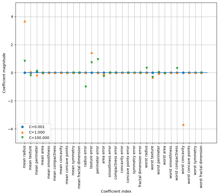
Linear Models for Multiclass Classification
Um aus einem binären Klassifizierungsalgorithmus einen für mehr als 2 Klassen zu machen, wird gerne die “Eine/r gegen den Rest”-Methode verwendet: Für jede Klasse wird ein binäres Modell gefittet, das zwischen dieser Klasse und den restlichen Klassen trennt. Zur Vorhersage werden die einzelnen Vorhersagen aller binären Modelle verglichen, und jenes mit dem größten Vorhersagewert gewinnt.
from sklearn.datasets import make_blobs

X, y = make_blobs(random_state=42)

mglearn.discrete_scatter(X[:, 0], X[:, 1], y)
plt.xlabel("Feature 0")
plt.ylabel("Feature 1")
plt.legend(["Class 0", "Class 1", "Class 2"])
plt.grid(True)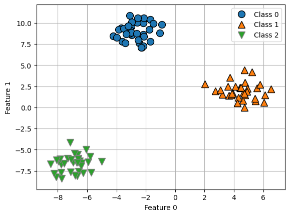
linear_svm = LinearSVC().fit(X, y)

print(f"Coefficient shape: {linear_svm.coef_.shape}")
print(f"Intercept   shape: {linear_svm.intercept_.shape}")
Coefficient shape: (3, 2)
Intercept shape: (3,)linear_svm.predict(np.array([[-2, 7],
[ 4, 2],
[-6, -5]]))array([0, 1, 2])logreg = LogisticRegression().fit(X, y)
print(f"Coefficient shape: {logreg.coef_.shape}")
print(f"Intercept shape: {logreg.intercept_.shape}")Coefficient shape: (3, 2)
Intercept shape: (3,)logreg.predict(np.array([[-2, 7],
[ 4, 2],
[-6, -5]]))array([0, 1, 2])mglearn.discrete_scatter(X[:, 0], X[:, 1], y)
if False:
mglearn.plots.plot_2d_classification(linear_svm, X, fill=True, alpha=.7)
line = np.linspace(-15, 15)
for coef, intercept, color in zip(linear_svm.coef_, linear_svm.intercept_, mglearn.cm3.colors):
plt.plot(line, -(line * coef[0] + intercept) / coef[1], c=color)
plt.ylim(-10, 15)
plt.xlim(-10, 8)
plt.xlabel("Feature 0")
plt.ylabel("Feature 1")
plt.legend(['Class 0', 'Class 1', 'Class 2',
'Line class 0', 'Line class 1', 'Line class 2'],
loc=(1.01, 0.3))
plt.grid(True)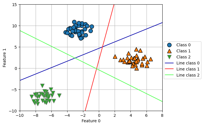
Decision Trees
Decision trees are widely used models for classification and regression tasks. Essentially, they learn a hierarchy of if/else questions, leading to a decision.
Graphviz
Zur graphischen Darstellung der Entscheidungsbäume verwenden wir die Software Graphviz und das gleichnamige Python-Paket graphviz. Diese können Sie mit folgenden Befehlen installieren:
- für das Python-Paket
pip install graphviz - für die Software Graphviz
conda install graphviz
Unter Windows müssen Sie anschließend den Graphviz-Installationsordner C:\Users\username\...\Anaconda3\Library\bin\graphviz der Umgebungsvariable PATH hinzufügen, damit die Software Graphviz gefunden wird.
import graphvizKlassifikation
Beispiel eines Entscheidungsbaums
mygraph = graphviz.Digraph(node_attr={'shape': 'box'},
                           edge_attr={'labeldistance': "10.5"},
                           format="png")
mygraph.node("0", "Has feathers?")
mygraph.node("1", "Can fly?")
mygraph.node("2", "Has fins?")
mygraph.node("3", "Hawk")
mygraph.node("4", "Penguin")
mygraph.node("5", "Dolphin")
mygraph.node("6", "Bear")
mygraph.edge("0", "1", label="True")
mygraph.edge("0", "2", label="False")
mygraph.edge("1", "3", label="True")
mygraph.edge("1", "4", label="False")
mygraph.edge("2", "5", label="True")
mygraph.edge("2", "6", label="False")
mygraph.render("tmp")

Image(filename='tmp.png')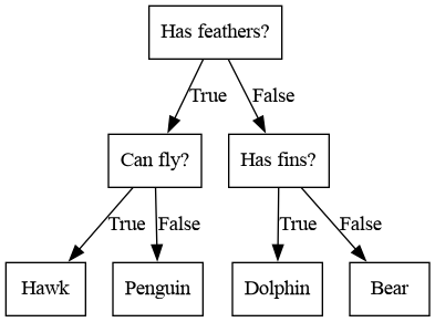
Beispiel: Synthetische 2D-Daten
from sklearn.tree import DecisionTreeClassifier
from sklearn.tree import export_graphviz
from sklearn.datasets import make_moons
Daten laden und in einem Scatterplot darstellen:
X, y = make_moons(n_samples=100, noise=0.25, random_state=3)

plt.figure(figsize=(6, 4))
mglearn.discrete_scatter(X[:, 0], X[:, 1], y)
plt.xlabel('feature 0')
plt.ylabel('feature 1')
plt.legend()
plt.grid(False)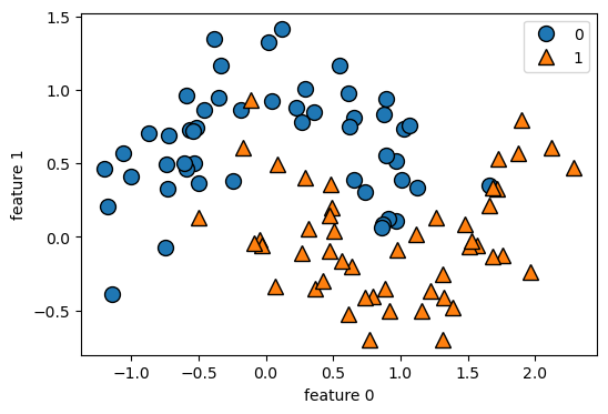
Funktion zur Darstellung eines Decision Tree Modells in Feature-Raum:
def plot_tree_partition(X, y, tree):
eps = X.std()/2.
x_min, x_max = X[:, 0].min() - eps, X[:, 0].max() + eps
y_min, y_max = X[:, 1].min() - eps, X[:, 1].max() + eps
xx = np.linspace(x_min, x_max, 1000)
yy = np.linspace(y_min, y_max, 1000)
X1, X2 = np.meshgrid(xx, yy)
X_grid = np.column_stack((X1.ravel(), X2.ravel()))
Z = tree.predict(X_grid)
Z = Z.reshape(X1.shape)
plt.contourf(X1, X2, Z, alpha=.4, levels=[0, .5, 1])
mglearn.discrete_scatter(X[:, 0], X[:, 1], y)
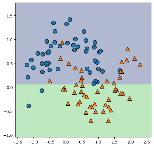
returnDecision Tree Modelle mit unterschiedlicher Verzweigungstiefe:
max_depth = 1

tree = DecisionTreeClassifier(max_depth=max_depth, random_state=0).fit(X, y)

export_graphviz(tree, out_file="tree.dot", class_names=["0", "1"], impurity=False)
my_file = open("tree.dot")
dot_graph = my_file.read()
my_file.close()
display(graphviz.Source(dot_graph))

plt.figure(figsize=(6, 6))
X_grid = plot_tree_partition(X, y, tree)
Controlling complexity of decision trees
max_depth… limit the maximum depth of the treemax_leaf_nodes… limit the maximum number of leavesmin_samples_split… require a minimum number of points in a node to keep splitting it
Beispiel: Brustkrebsdaten
from sklearn.datasets import load_breast_cancer
cancer = load_breast_cancer()

from sklearn.model_selection import train_test_split
X_train, X_test, y_train, y_test = train_test_split(
    cancer.data, cancer.target, stratify=cancer.target, random_state=42)

tree = DecisionTreeClassifier(random_state=0)
tree.fit(X_train, y_train)

print(f"Accuracy on training set: {tree.score(X_train, y_train):.3f}")
print(f"Accuracy on     test set: {tree.score(X_test, y_test):.3f}")
Accuracy on training set: 1.000
Accuracy on test set: 0.937tree = DecisionTreeClassifier(max_depth=4, random_state=0)
tree.fit(X_train, y_train)
print(f"Accuracy on training set: {tree.score(X_train, y_train):.3f}")
print(f"Accuracy on test set: {tree.score(X_test, y_test):.3f}")Accuracy on training set: 0.988
Accuracy on test set: 0.951export_graphviz(tree, out_file="tree.dot", class_names=["malignant", "benign"],
feature_names=cancer.feature_names, impurity=False, filled=True)
my_file = open("tree.dot")
dot_graph = my_file.read()
my_file.close()
display(graphviz.Source(dot_graph))
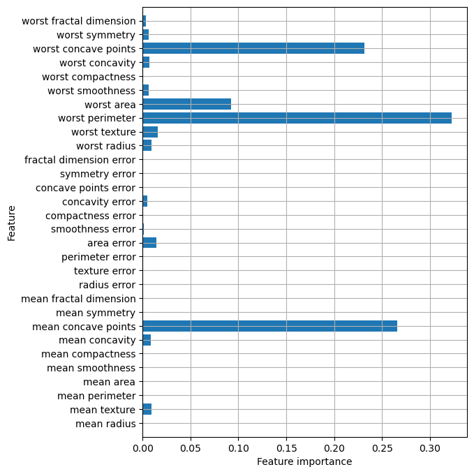
Feature Importance
Feature Importance rates how important each feature is for the decision a tree makes. It is a number between 0 and 1 for each feature, where 0 means “not used at all” and 1 means “perfectly predicts the target.” The feature importances always sum to 1.
If a feature has a low feature_importance, it doesn’t mean that this feature is uninformative. It only means that the feature was not picked by the tree, likely because another feature encodes the same information.
In contrast to the coefficients in linear models, feature importances are always positive, and don’t encode which class a feature is indicative of.
Beispiel: Brustkrebsdaten
tree.feature_importances_array([0. , 0. , 0. , 0. , 0. ,
0. , 0. , 0. , 0. , 0. ,
0.01019737, 0.04839825, 0. , 0. , 0.0024156 ,
0. , 0. , 0. , 0. , 0. ,
0.72682851, 0.0458159 , 0. , 0. , 0.0141577 ,
0. , 0.018188 , 0.1221132 , 0.01188548, 0. ])plt.figure(figsize=(6, 8))
n_features = cancer.data.shape[1]
plt.barh(range(n_features), tree.feature_importances_, align='center')
plt.yticks(np.arange(n_features), cancer.feature_names)
plt.xlabel("Feature importance")
plt.ylabel("Feature")
plt.ylim(-1, n_features)
plt.grid(True)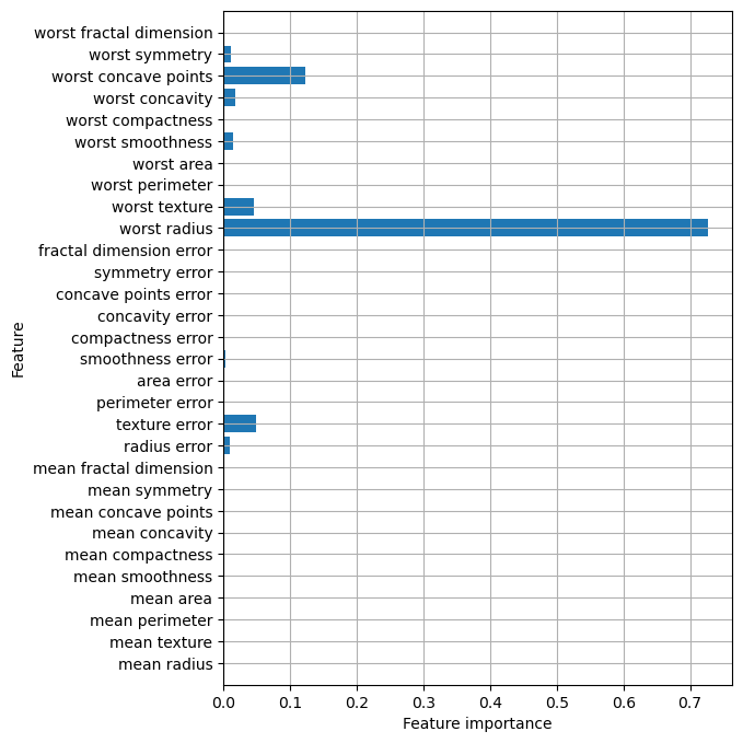
Beispiel: synthetisch
tree = mglearn.plots.plot_tree_not_monotone()
display(tree);
Feature importances: [0. 1.]
Regression
ram_prices = pd.read_csv("daten/ram_price.csv", index_col=0)
ram_prices.head()| date | price | |
|---|---|---|
| 0 | 1957.0 | 411041792.0 |
| 1 | 1959.0 | 67947725.0 |
| 2 | 1960.0 | 5242880.0 |
| 3 | 1965.0 | 2642412.0 |
| 4 | 1970.0 | 734003.0 |
plt.figure(figsize=(8, 6))
plt.semilogy(ram_prices.date, ram_prices.price, '.-')
plt.xlabel("Year")
plt.ylabel("Price in $/Mbyte")
plt.grid(True)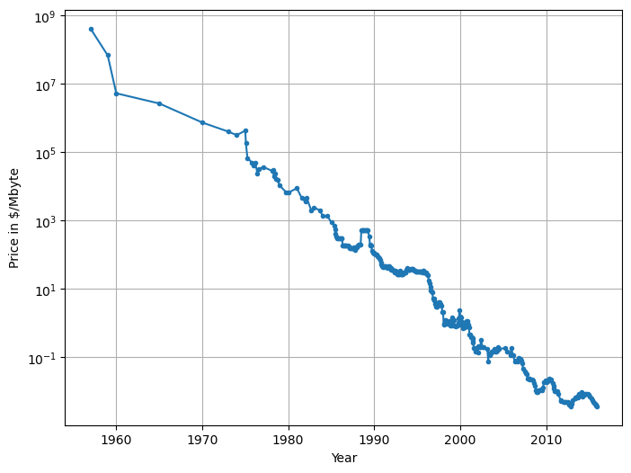
from sklearn.tree import DecisionTreeRegressor
from sklearn.linear_model import LinearRegression

# Use historical data to forecast prices after the year 2000
data_train = ram_prices[ram_prices.date < 2000]
data_test  = ram_prices[ram_prices.date >= 2000]

# predict prices based on date:
X_train = np.reshape(data_train.date.values, (-1, 1))
# we use a log-transform to get a simpler relationship of data to target
y_train = np.log(data_train.price)

tree       = DecisionTreeRegressor(max_depth=None).fit(X_train, y_train)
#tree       = DecisionTreeRegressor(max_depth=2).fit(X_train, y_train)
linear_reg = LinearRegression().fit(X_train, y_train)

# predict on all data
X_all = np.reshape(ram_prices.date.values, (-1, 1))

pred_tree = tree.predict(X_all)
pred_lr   = linear_reg.predict(X_all)

# undo log-transform
price_tree = np.exp(pred_tree)
price_lr = np.exp(pred_lr)plt.figure(figsize=(8,6))
plt.semilogy(data_train.date, data_train.price, label="training data")
plt.semilogy(data_test.date , data_test.price , label="test data")
plt.semilogy(ram_prices.date, price_tree , '.-', label="tree prediction")
plt.semilogy(ram_prices.date, price_lr , '--', label="linear prediction")
plt.legend()
plt.grid(True)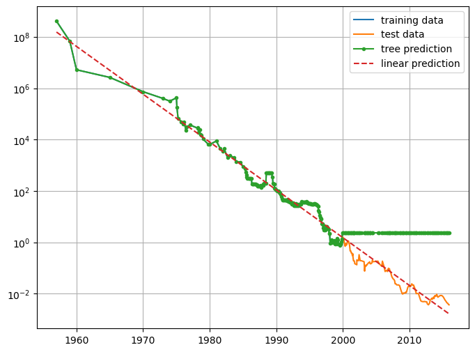
The DecisionTreeRegressor is not able to extrapolate. It is actually possible to make very good forecasts with tree-based models (for example, when trying to predict whether a price will go up or down). The point of this example was not to show that trees are a bad model for time series, but to illustrate a particular property of how trees make predictions.
Ensembles of Decision Trees
The main downside of decision trees is that they tend to overfit and provide poor generalization performance. Therefore, in most applications, ensemble methods are usually used in place of a single decision tree.
Random forests
A random forest is a collection of decision trees, where each tree is slightly different from the others.
Parameters:
n_estimators… number of treesmax_features… number of features in each node that are randomly selected
To make a prediction using the random forest, the algorithm first makes a prediction for every tree in the forest. For regression, we can average these results to get our final prediction. For classification, a “soft voting” strategy is used.
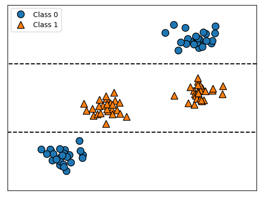
Beispiel Moon Data:
from sklearn.ensemble import RandomForestClassifier
from sklearn.datasets import make_moons

X, y = make_moons(n_samples=100, noise=0.25, random_state=3)
X_train, X_test, y_train, y_test = train_test_split(X, y, stratify=y,
                                                    random_state=42)

forest = RandomForestClassifier(n_estimators=5, random_state=2)
forest.fit(X_train, y_train)

print(f"Training set score: {forest.score(X_train, y_train):.2f}")
print(f"    Test set score: {forest.score(X_test, y_test):.2f}")
Training set score: 0.96
Test set score: 0.92fig, axes = plt.subplots(2, 3, figsize=(20, 10))
for i, (ax, tree) in enumerate(zip(axes.ravel(), forest.estimators_)):
ax.set_title(f"Tree {i}")
mglearn.plots.plot_tree_partition(X_train, y_train, tree, ax=ax)
mglearn.plots.plot_2d_separator(forest, X_train, fill=True, ax=axes[-1, -1],
alpha=.4)
axes[-1, -1].set_title("Random Forest")
mglearn.discrete_scatter(X_train[:, 0], X_train[:, 1], y_train);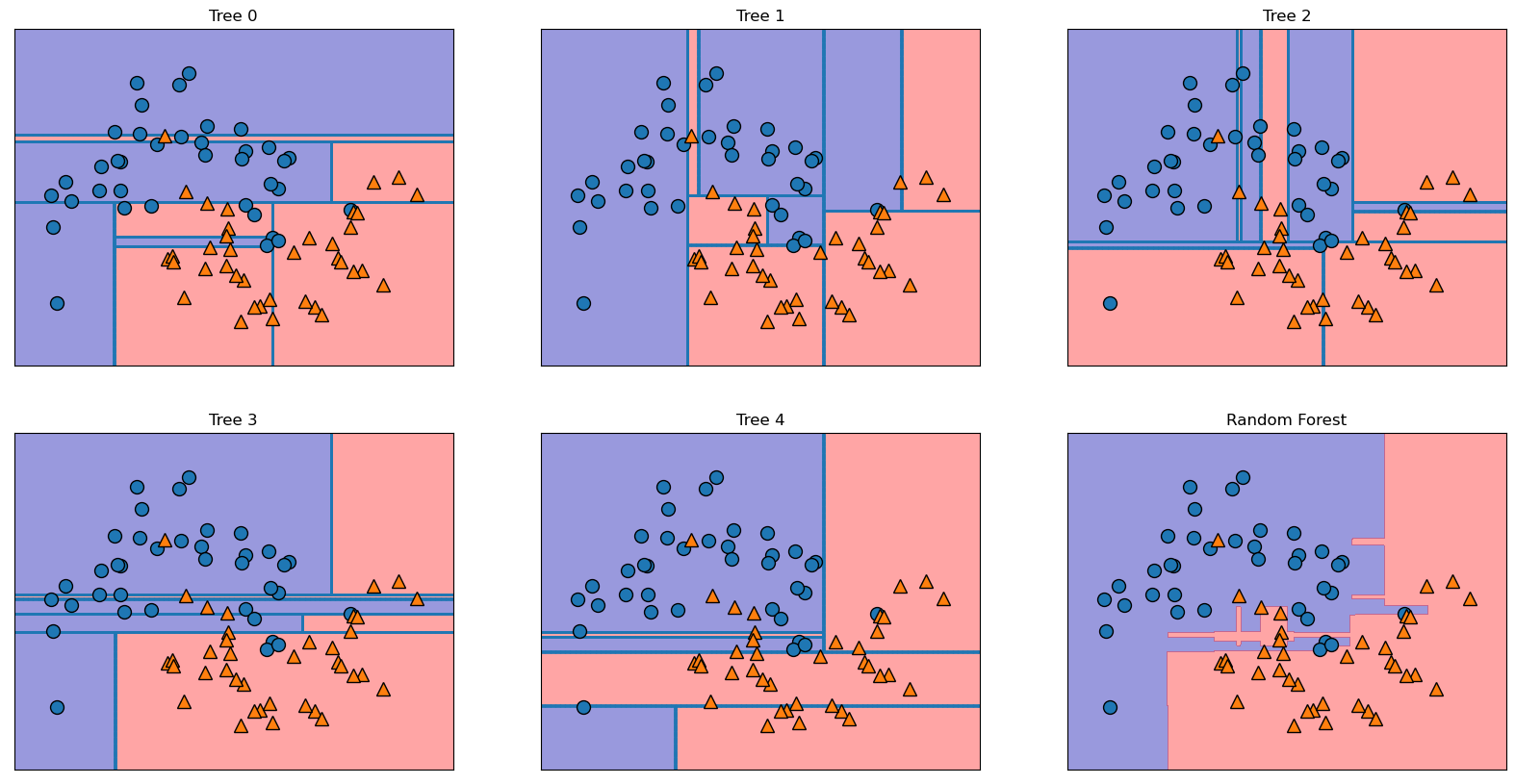
Beispiel Brustkresbsdaten:
X_train, X_test, y_train, y_test = train_test_split(
    cancer.data, cancer.target, random_state=0)

forest = RandomForestClassifier(n_estimators=100, random_state=0)
forest.fit(X_train, y_train)

print(f"Accuracy on training set: {forest.score(X_train, y_train):.3f}")
print(f"Accuracy on     test set: {forest.score(X_test, y_test):.3f}")
Accuracy on training set: 1.000
Accuracy on test set: 0.972plt.figure(figsize=(6, 8))
n_features = cancer.data.shape[1]
plt.barh(range(n_features), forest.feature_importances_, align='center')
plt.yticks(np.arange(n_features), cancer.feature_names)
plt.xlabel("Feature importance")
plt.ylabel("Feature")
plt.ylim(-1, n_features)
plt.grid(True)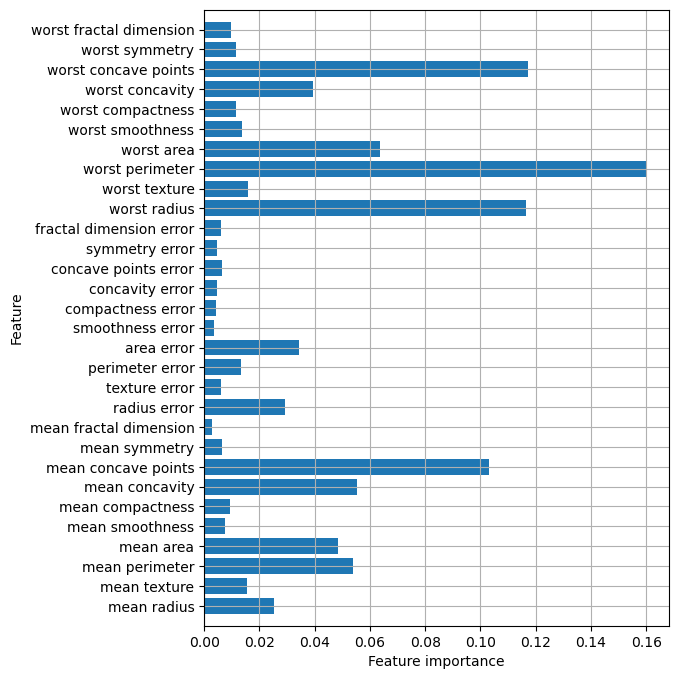
The randomness in building the random forest forces the algorithm to consider many possible explanations, the result being that the random forest captures a much broader picture of the data than a single tree.
Gradient Boosted Trees (Gradient Boosting Machines)
Build trees in a serial manner, where each tree tries to correct the mistakes of the previous one.
Parameters:
max_depthlearning_rate… controls how strongly each tree tries to correct the mistakes of the previous treesn_estimators
Beispiel Brustkresbsdaten:
from sklearn.ensemble import GradientBoostingClassifier

X_train, X_test, y_train, y_test = train_test_split(
    cancer.data, cancer.target, random_state=0)
gbrt = GradientBoostingClassifier(random_state=0)
gbrt.fit(X_train, y_train)
print(f"Accuracy on training set: {gbrt.score(X_train, y_train):.3f}")
print(f"Accuracy on test set: {gbrt.score(X_test, y_test):.3f}")Accuracy on training set: 1.000
Accuracy on test set: 0.965gbrt = GradientBoostingClassifier(random_state=0, max_depth=1)
gbrt.fit(X_train, y_train)
print(f"Accuracy on training set: {gbrt.score(X_train, y_train):.3f}")
print(f"Accuracy on test set: {gbrt.score(X_test, y_test):.3f}")Accuracy on training set: 0.991
Accuracy on test set: 0.972gbrt = GradientBoostingClassifier(random_state=0, learning_rate=0.01)
gbrt.fit(X_train, y_train)
print(f"Accuracy on training set: {gbrt.score(X_train, y_train):.3f}")
print(f"Accuracy on test set: {gbrt.score(X_test, y_test):.3f}")Accuracy on training set: 0.988
Accuracy on test set: 0.965gbrt = GradientBoostingClassifier(random_state=0, max_depth=1)
gbrt.fit(X_train, y_train)
plt.figure(figsize=(6, 8))
n_features = cancer.data.shape[1]
plt.barh(range(n_features), gbrt.feature_importances_, align='center')
plt.yticks(np.arange(n_features), cancer.feature_names)
plt.xlabel("Feature importance")
plt.ylabel("Feature")
plt.ylim(-1, n_features)
plt.grid(True)