import pandas as pd
import matplotlib.pyplot as plt
import numpy as np
import mglearnEngineering Features
Book
This IPython notebook follows the book Introduction to Machine Learning with Python by Andreas Mueller and Sarah Guido and uses material from its github repository and from the working files of the training course Advanced Machine Learning with scikit-learn. Excerpts taken from the book are displayed in italic letters.
The contents of this Jupyter notebook corresponds in the book Introduction to Machine Learning with Python to:
- Chapter 4 “Representing Data and Engineering Features”: p. 211 to 250
Python
from pandas.plotting import register_matplotlib_converters
register_matplotlib_converters()
if 0:
import warnings
warnings.filterwarnings("ignore")Categorical Variables
data = pd.read_csv("daten/adult_data.csv", sep=',', skipinitialspace=True,
                   names=['age', 'workclass', 'fnlwgt', 'education',  'education-num',
                   'marital-status', 'occupation', 'relationship', 'race', 'gender',
                   'capital-gain', 'capital-loss', 'hours-per-week', 'native-country',
                   'income'])

# For illustration purposes, we only select some of the columns:
data = data[['age', 'workclass', 'education', 'gender', 'hours-per-week',
             'occupation', 'income']]

# IPython.display allows nice output formatting within the Jupyter notebook
data.head()| age | workclass | education | gender | hours-per-week | occupation | income | |
|---|---|---|---|---|---|---|---|
| 0 | 39 | State-gov | Bachelors | Male | 40 | Adm-clerical | <=50K |
| 1 | 50 | Self-emp-not-inc | Bachelors | Male | 13 | Exec-managerial | <=50K |
| 2 | 38 | Private | HS-grad | Male | 40 | Handlers-cleaners | <=50K |
| 3 | 53 | Private | 11th | Male | 40 | Handlers-cleaners | <=50K |
| 4 | 28 | Private | Bachelors | Female | 40 | Prof-specialty | <=50K |
Checking string-encoded categorical data
data['gender'].value_counts()Male 21790
Female 10771
Name: gender, dtype: int64print(f"Original features:\n\n{list(data.columns)} \n")
data_dummies = pd.get_dummies(data)
print(f"Features after get_dummies:\n\n{list(data_dummies.columns)}")Original features:
['age', 'workclass', 'education', 'gender', 'hours-per-week', 'occupation', 'income']
Features after get_dummies:
['age', 'hours-per-week', 'workclass_?', 'workclass_Federal-gov', 'workclass_Local-gov', 'workclass_Never-worked', 'workclass_Private', 'workclass_Self-emp-inc', 'workclass_Self-emp-not-inc', 'workclass_State-gov', 'workclass_Without-pay', 'education_10th', 'education_11th', 'education_12th', 'education_1st-4th', 'education_5th-6th', 'education_7th-8th', 'education_9th', 'education_Assoc-acdm', 'education_Assoc-voc', 'education_Bachelors', 'education_Doctorate', 'education_HS-grad', 'education_Masters', 'education_Preschool', 'education_Prof-school', 'education_Some-college', 'gender_Female', 'gender_Male', 'occupation_?', 'occupation_Adm-clerical', 'occupation_Armed-Forces', 'occupation_Craft-repair', 'occupation_Exec-managerial', 'occupation_Farming-fishing', 'occupation_Handlers-cleaners', 'occupation_Machine-op-inspct', 'occupation_Other-service', 'occupation_Priv-house-serv', 'occupation_Prof-specialty', 'occupation_Protective-serv', 'occupation_Sales', 'occupation_Tech-support', 'occupation_Transport-moving', 'income_<=50K', 'income_>50K']data_dummies.head(3)| age | hours-per-week | workclass_? | workclass_Federal-gov | workclass_Local-gov | workclass_Never-worked | workclass_Private | workclass_Self-emp-inc | workclass_Self-emp-not-inc | workclass_State-gov | ... | occupation_Machine-op-inspct | occupation_Other-service | occupation_Priv-house-serv | occupation_Prof-specialty | occupation_Protective-serv | occupation_Sales | occupation_Tech-support | occupation_Transport-moving | income_<=50K | income_>50K | |
|---|---|---|---|---|---|---|---|---|---|---|---|---|---|---|---|---|---|---|---|---|---|
| 0 | 39 | 40 | 0 | 0 | 0 | 0 | 0 | 0 | 0 | 1 | ... | 0 | 0 | 0 | 0 | 0 | 0 | 0 | 0 | 1 | 0 |
| 1 | 50 | 13 | 0 | 0 | 0 | 0 | 0 | 0 | 1 | 0 | ... | 0 | 0 | 0 | 0 | 0 | 0 | 0 | 0 | 1 | 0 |
| 2 | 38 | 40 | 0 | 0 | 0 | 0 | 1 | 0 | 0 | 0 | ... | 0 | 0 | 0 | 0 | 0 | 0 | 0 | 0 | 1 | 0 |
3 rows × 46 columns
# Get only the columns containing features
# that is all columns from 'age' to 'occupation_ Transport-moving'
# This range contains all the features but not the target
features = data_dummies.loc[:, 'age':'occupation_Transport-moving']

# extract NumPy arrays
X = features.values
y = data_dummies['income_>50K'].values
print(f"X.shape: {X.shape}  y.shape: {y.shape}")
X.shape: (32561, 44) y.shape: (32561,)from sklearn.linear_model import LogisticRegression
from sklearn.model_selection import train_test_split
X_train, X_test, y_train, y_test = train_test_split(X, y, random_state=0)
logreg = LogisticRegression(solver='liblinear')
logreg.fit(X_train, y_train)
print(f"Test score: {logreg.score(X_test, y_test):.2f}")Test score: 0.81Numbers can encode categoricals
# create a dataframe with an integer feature and a categorical string feature
demo_df = pd.DataFrame({'Integer Feature': [0, 1, 2, 1],
                        'Categorical Feature': ['socks', 'fox', 'socks', 'box']})
demo_df| Integer Feature | Categorical Feature | |
|---|---|---|
| 0 | 0 | socks |
| 1 | 1 | fox |
| 2 | 2 | socks |
| 3 | 1 | box |
pd.get_dummies(demo_df)| Integer Feature | Categorical Feature_box | Categorical Feature_fox | Categorical Feature_socks | |
|---|---|---|---|---|
| 0 | 0 | 0 | 0 | 1 |
| 1 | 1 | 0 | 1 | 0 |
| 2 | 2 | 0 | 0 | 1 |
| 3 | 1 | 1 | 0 | 0 |
pd.get_dummies(demo_df, columns=['Integer Feature', 'Categorical Feature'])| Integer Feature_0 | Integer Feature_1 | Integer Feature_2 | Categorical Feature_box | Categorical Feature_fox | Categorical Feature_socks | |
|---|---|---|---|---|---|---|
| 0 | 1 | 0 | 0 | 0 | 0 | 1 |
| 1 | 0 | 1 | 0 | 0 | 1 | 0 |
| 2 | 0 | 0 | 1 | 0 | 0 | 1 |
| 3 | 0 | 1 | 0 | 1 | 0 | 0 |
Binning, Discretization, Linear Models and Trees
from sklearn.linear_model import LinearRegression
from sklearn.tree         import DecisionTreeRegressor

X, y = mglearn.datasets.make_wave(n_samples=100)
line = np.linspace(-3, 3, 1000, endpoint=False).reshape(-1, 1)

plt.figure(figsize=(8,6))

reg = DecisionTreeRegressor(min_samples_split=3).fit(X, y)
plt.plot(line, reg.predict(line), label="decision tree")

reg = LinearRegression().fit(X, y)
plt.plot(line, reg.predict(line), label="linear regression")

plt.plot(X[:, 0], y, 'o', c='k')
plt.ylabel("target")
plt.xlabel("feature")
plt.legend(loc="best")
plt.grid(True)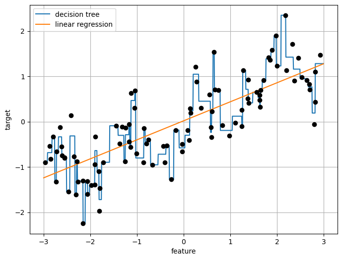
bins = np.linspace(-3, 3, 11)
print(f"bins: {bins}")
bins: [-3. -2.4 -1.8 -1.2 -0.6 0. 0.6 1.2 1.8 2.4 3. ]which_bin = np.digitize(X, bins=bins)
print(f"Data points:\n{X[:5]}\n")
print(f"Bin membership for data points:\n{which_bin[:5]}")Data points:
[[-0.75275929]
[ 2.70428584]
[ 1.39196365]
[ 0.59195091]
[-2.06388816]]
Bin membership for data points:
[[ 4]
[10]
[ 8]
[ 6]
[ 2]]np.unique(which_bin)array([ 1, 2, 3, 4, 5, 6, 7, 8, 9, 10])# transform using the OneHotEncoder:
from sklearn.preprocessing import OneHotEncoder
# configure the OneHotEncoder:
encoder = OneHotEncoder(sparse_output=False, categories='auto')
# encoder.fit finds the unique values that appear in which_bin
encoder.fit(which_bin)
# transform creates the one-hot encoding
X_binned = encoder.transform(which_bin)
print(X_binned[:5])[[0. 0. 0. 1. 0. 0. 0. 0. 0. 0.]
[0. 0. 0. 0. 0. 0. 0. 0. 0. 1.]
[0. 0. 0. 0. 0. 0. 0. 1. 0. 0.]
[0. 0. 0. 0. 0. 1. 0. 0. 0. 0.]
[0. 1. 0. 0. 0. 0. 0. 0. 0. 0.]]line_binned = encoder.transform(np.digitize(line, bins=bins))
plt.figure(figsize=(8,6))
reg = LinearRegression().fit(X_binned, y)
plt.plot(line, reg.predict(line_binned), label='linear regression binned')
reg = DecisionTreeRegressor(min_samples_split=3).fit(X_binned, y)
plt.plot(line, reg.predict(line_binned), label='decision tree binned')
plt.plot(X[:, 0], y, 'o', c='k')
plt.vlines(bins, -3, 3, linewidth=1, alpha=.2)
plt.legend(loc="best")
plt.ylabel("traget")
plt.xlabel("feature");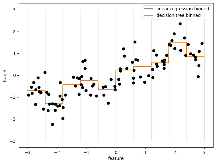
Interactions and Polynomials
Interactions
X_combined = np.hstack([X, X_binned])
print(X_combined[:5])
[[-0.75275929 0. 0. 0. 1. 0.
0. 0. 0. 0. 0. ]
[ 2.70428584 0. 0. 0. 0. 0.
0. 0. 0. 0. 1. ]
[ 1.39196365 0. 0. 0. 0. 0.
0. 0. 1. 0. 0. ]
[ 0.59195091 0. 0. 0. 0. 0.
1. 0. 0. 0. 0. ]
[-2.06388816 0. 1. 0. 0. 0.
0. 0. 0. 0. 0. ]]reg = LinearRegression().fit(X_combined, y)
line_combined = np.hstack([line, line_binned])
plt.figure(figsize=(8,6))
plt.plot(line, reg.predict(line_combined),
linewidth=2, c='r',
label='linear regression combined')
for bin in bins:
plt.plot([bin, bin], [-3, 3], ':', c='k')
plt.legend(loc="best")
plt.ylabel("Regression output")
plt.xlabel("Input feature")
plt.plot(X[:, 0], y, 'o', c='k');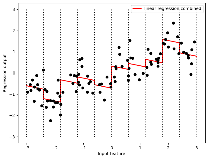
Because the slope is shared across all bins, it doesn’t seem to be very helpful. We would rather have a separate slope for each bin! We can achieve this by adding an interaction or product feature that indicates which bin a data point is in and where it lies on the x-axis.
X_product = np.hstack([X_binned, X*X_binned])
print(X_product.shape)
print(X_product[:5])
(100, 20)
[[ 0. 0. 0. 1. 0. 0.
0. 0. 0. 0. -0. -0.
-0. -0.75275929 -0. -0. -0. -0.
-0. -0. ]
[ 0. 0. 0. 0. 0. 0.
0. 0. 0. 1. 0. 0.
0. 0. 0. 0. 0. 0.
0. 2.70428584]
[ 0. 0. 0. 0. 0. 0.
0. 1. 0. 0. 0. 0.
0. 0. 0. 0. 0. 1.39196365
0. 0. ]
[ 0. 0. 0. 0. 0. 1.
0. 0. 0. 0. 0. 0.
0. 0. 0. 0.59195091 0. 0.
0. 0. ]
[ 0. 1. 0. 0. 0. 0.
0. 0. 0. 0. -0. -2.06388816
-0. -0. -0. -0. -0. -0.
-0. -0. ]]reg = LinearRegression().fit(X_product, y)
line_product = np.hstack([line_binned, line*line_binned])
plt.plot(line, reg.predict(line_product),
linewidth=2, c='r',
label='linear regression product')
for bin in bins:
plt.plot([bin, bin], [-3, 3], ':', c='k')
plt.plot(X[:, 0], y, 'o', c='k')
plt.ylabel("Regression output")
plt.xlabel("Input feature")
plt.legend(loc="best");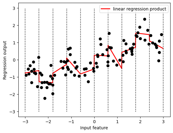
Polynomials
Another way to expand a continuous feature is to use polynomials of the original features.
from sklearn.preprocessing import PolynomialFeatures

# include polynomials up to x**10:
# the default "include_bias=True" adds a features that's constantly 1
poly = PolynomialFeatures(degree=10, include_bias=True)
poly.fit(X)
X_poly = poly.transform(X)

print(poly.get_feature_names_out())
['1' 'x0' 'x0^2' 'x0^3' 'x0^4' 'x0^5' 'x0^6' 'x0^7' 'x0^8' 'x0^9' 'x0^10']print(f"First 5 entries of X:\n{X[:5]}")
print(f"First 5 entries of X_poly:\n{X_poly[:5]}")First 5 entries of X:
[[-0.75275929]
[ 2.70428584]
[ 1.39196365]
[ 0.59195091]
[-2.06388816]]
First 5 entries of X_poly:
[[ 1.00000000e+00 -7.52759287e-01 5.66646544e-01 -4.26548448e-01
3.21088306e-01 -2.41702204e-01 1.81943579e-01 -1.36959719e-01
1.03097700e-01 -7.76077513e-02 5.84199555e-02]
[ 1.00000000e+00 2.70428584e+00 7.31316190e+00 1.97768801e+01
5.34823369e+01 1.44631526e+02 3.91124988e+02 1.05771377e+03
2.86036036e+03 7.73523202e+03 2.09182784e+04]
[ 1.00000000e+00 1.39196365e+00 1.93756281e+00 2.69701700e+00
3.75414962e+00 5.22563982e+00 7.27390068e+00 1.01250053e+01
1.40936394e+01 1.96178338e+01 2.73073115e+01]
[ 1.00000000e+00 5.91950905e-01 3.50405874e-01 2.07423074e-01
1.22784277e-01 7.26822637e-02 4.30243318e-02 2.54682921e-02
1.50759786e-02 8.92423917e-03 5.28271146e-03]
[ 1.00000000e+00 -2.06388816e+00 4.25963433e+00 -8.79140884e+00
1.81444846e+01 -3.74481869e+01 7.72888694e+01 -1.59515582e+02
3.29222321e+02 -6.79478050e+02 1.40236670e+03]]reg = LinearRegression().fit(X_poly, y)
line_poly = poly.transform(line)
plt.figure(figsize=(8,6))
plt.plot(line, reg.predict(line_poly), label='polynomial linear regression')
plt.plot(X[:, 0], y, 'o', c='k')
plt.ylabel("Regression output")
plt.xlabel("Input feature")
plt.legend(loc="best")
plt.grid(True)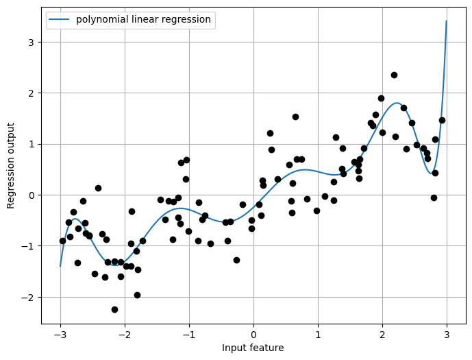
Realworld Example: Boston Housing dataset
from sklearn.model_selection import train_test_split
from sklearn.preprocessing   import MinMaxScaler

# from sklearn.datasets        import load_boston
# boston = load_boston()
data_url = "http://lib.stat.cmu.edu/datasets/boston"
raw_df = pd.read_csv(data_url, sep="\s+", skiprows=22, header=None)
X = np.hstack([raw_df.values[::2, :], raw_df.values[1::2, :2]])
y = raw_df.values[1::2, 2]

X_train, X_test, y_train, y_test = train_test_split(X, y, random_state=0)

# rescale data:
scaler = MinMaxScaler()
X_train_scaled = scaler.fit_transform(X_train)
X_test_scaled  = scaler.transform(X_test)
poly = PolynomialFeatures(degree=2).fit(X_train_scaled)
X_train_poly = poly.transform(X_train_scaled)
X_test_poly = poly.transform(X_test_scaled)
print(f"X_train.shape: {X_train.shape}") # 1 + 13 + 13*14/2
print(f"X_train_poly.shape: {X_train_poly.shape}")
print(poly.get_feature_names_out())X_train.shape: (379, 13)
X_train_poly.shape: (379, 105)
['1' 'x0' 'x1' 'x2' 'x3' 'x4' 'x5' 'x6' 'x7' 'x8' 'x9' 'x10' 'x11' 'x12'
'x0^2' 'x0 x1' 'x0 x2' 'x0 x3' 'x0 x4' 'x0 x5' 'x0 x6' 'x0 x7' 'x0 x8'
'x0 x9' 'x0 x10' 'x0 x11' 'x0 x12' 'x1^2' 'x1 x2' 'x1 x3' 'x1 x4' 'x1 x5'
'x1 x6' 'x1 x7' 'x1 x8' 'x1 x9' 'x1 x10' 'x1 x11' 'x1 x12' 'x2^2' 'x2 x3'
'x2 x4' 'x2 x5' 'x2 x6' 'x2 x7' 'x2 x8' 'x2 x9' 'x2 x10' 'x2 x11'
'x2 x12' 'x3^2' 'x3 x4' 'x3 x5' 'x3 x6' 'x3 x7' 'x3 x8' 'x3 x9' 'x3 x10'
'x3 x11' 'x3 x12' 'x4^2' 'x4 x5' 'x4 x6' 'x4 x7' 'x4 x8' 'x4 x9' 'x4 x10'
'x4 x11' 'x4 x12' 'x5^2' 'x5 x6' 'x5 x7' 'x5 x8' 'x5 x9' 'x5 x10'
'x5 x11' 'x5 x12' 'x6^2' 'x6 x7' 'x6 x8' 'x6 x9' 'x6 x10' 'x6 x11'
'x6 x12' 'x7^2' 'x7 x8' 'x7 x9' 'x7 x10' 'x7 x11' 'x7 x12' 'x8^2' 'x8 x9'
'x8 x10' 'x8 x11' 'x8 x12' 'x9^2' 'x9 x10' 'x9 x11' 'x9 x12' 'x10^2'
'x10 x11' 'x10 x12' 'x11^2' 'x11 x12' 'x12^2']from sklearn.linear_model import Ridge
ridge = Ridge().fit(X_train_scaled, y_train)
print(f"test score without interactions: {ridge.score(X_test_scaled, y_test):.3f}")
ridge = Ridge().fit(X_train_poly, y_train)
print(f"test score with interactions: {ridge.score(X_test_poly, y_test):.3f}")test score without interactions: 0.621
test score with interactions: 0.753from sklearn.ensemble import RandomForestRegressor
rf = RandomForestRegressor(n_estimators=100).fit(X_train_scaled, y_train)
print(f"test score without interactions: {rf.score(X_test_scaled, y_test):.3f}")
rf = RandomForestRegressor(n_estimators=100).fit(X_train_poly, y_train)
print(f"test score with interactions: {rf.score(X_test_poly, y_test):.3f}")test score without interactions: 0.789
test score with interactions: 0.772Note: As you saw in the previous examples, binning, polynomials, and interactions can have a huge influence on how models perform on a given dataset. This is particularly true for less complex models like linear models. Tree-based models, on the other hand, are often able to discover important interactions themselves, and don’t require transforming the data explicitly most of the time.
Automatic Feature Selection
Adding features makes models more complex, and so increases the chance of overfitting. Reducing the number of features to only the most useful ones can lead to simpler models that generalize better.
Univariate Statistics
consider each feature individually.
from sklearn.datasets import load_breast_cancer
from sklearn.feature_selection import SelectPercentile
from sklearn.model_selection import train_test_split

cancer = load_breast_cancer()

# get deterministic random numbers
rng = np.random.RandomState(42)
noise = rng.normal(size=(len(cancer.data), 50))

# add noise features to the data
# the first 30 features are from the dataset, the next 50 are noise
X_w_noise = np.hstack([cancer.data, noise])

X_train, X_test, y_train, y_test = train_test_split(
    X_w_noise, cancer.target, random_state=0, test_size=.5)

# use SelectPercentile to select 50 % of features:
select = SelectPercentile(percentile=50)
select.fit(X_train, y_train)

# transform training set:
X_train_selected = select.transform(X_train)

print(f"X_train.shape: {X_train.shape}")
print(f"X_train_selected.shape: {X_train_selected.shape}")
X_train.shape: (284, 80)
X_train_selected.shape: (284, 40)mask = select.get_support()
print(mask)
# visualize the mask. black is True, white is False
plt.matshow(mask.reshape(1, -1), cmap='gray_r')
plt.xlabel("Sample index");[ True True True True True True True True True False True False
True True True True True True False False True True True True
True True True True True True False False False True False True
False False True False False False False True False False True False
False True False True False False False False False False True False
True False False False False True False True False False False False
True True False True False False False False]
from sklearn.linear_model import LogisticRegression

# transform test data:
X_test_selected = select.transform(X_test)

lr = LogisticRegression(solver='liblinear')

lr.fit(X_train, y_train)
print(f"Test score with all features: {lr.score(X_test, y_test):.3f}")

lr.fit(X_train_selected, y_train)
print(f"Test score with only selected features: {lr.score(X_test_selected, y_test):.3f}")
Test score with all features: 0.930
Test score with only selected features: 0.940Model-based Feature Selection
considers all features at once, and so can capture interactions.
from sklearn.feature_selection import SelectFromModel
from sklearn.ensemble import RandomForestClassifier

select = SelectFromModel(RandomForestClassifier(n_estimators=100, random_state=42),
                         threshold="median")

select.fit(X_train, y_train)
X_train_selected = select.transform(X_train)
print(f"X_train.shape: {X_train.shape}")
print(f"X_train_selected.shape: {X_train_selected.shape}")
X_train.shape: (284, 80)
X_train_selected.shape: (284, 40)mask = select.get_support()
# visualize the mask. black is True, white is False
plt.matshow(mask.reshape(1, -1), cmap='gray_r')
plt.xlabel("Sample index");
X_test_selected = select.transform(X_test)
score = LogisticRegression(solver='liblinear').fit(X_train_selected, y_train).score(X_test_selected, y_test)
print(f"Test score Model-based Feature Selection: {score:.3f}")
Test score Model-based Feature Selection: 0.951Iterative feature selection
a series of models are built, with varying numbers of features.
Recursive feature elimination (RFE) starts with all features, builds a model, and discards the least important feature according to the model. Then a new model is built using all but the discarded feature, and so on until only a prespecified number of features are left.
from sklearn.feature_selection import RFE

select = RFE(RandomForestClassifier(n_estimators=100, random_state=2),
             n_features_to_select=40)

select.fit(X_train, y_train)
RFE(estimator=RandomForestClassifier(random_state=2), n_features_to_select=40)In a Jupyter environment, please rerun this cell to show the HTML representation or trust the notebook.
On GitHub, the HTML representation is unable to render, please try loading this page with nbviewer.org.
RFE(estimator=RandomForestClassifier(random_state=2), n_features_to_select=40)
RandomForestClassifier(random_state=2)
RandomForestClassifier(random_state=2)
# visualize the selected features:
mask = select.get_support()
plt.matshow(mask.reshape(1, -1), cmap='gray_r')
plt.xlabel("Sample index");
X_train_rfe = select.transform(X_train)
X_test_rfe  = select.transform(X_test)

score = LogisticRegression(solver='liblinear').fit(X_train_rfe, y_train).score(X_test_rfe, y_test)
print(f"Test score of LogisticRegression with RFE: {score:.10f}")

# mit select-Algorithmus:
# = RandomForestClassifier(n_estimators=100, random_state=2).fit(X_train_rfe, y_train).score(X_test_rfe, y_test)
print(f"Test score with select: {select.score(X_test, y_test):.10f}")
Test score of LogisticRegression with RFE: 0.9543859649
Test score with select: 0.9403508772Utilizing Expert Knowledge - Example
In New York, Citi Bike operates a network of bicycle rental stations with a subscription system. The stations are all over the city and provide a convenient way to get around. Bike rental data is made public in an anonymized form and has been analyzed in various ways. The task we want to solve is to predict for a given time and day how many people will rent a bike in front of Andreas’s house—so he knows if any bikes will be left for him.
# load an preprocess:
data_raw = pd.read_csv("daten/citibike.csv")
data_raw.head(5)| tripduration | starttime | stoptime | start station id | start station name | start station latitude | start station longitude | end station id | end station name | end station latitude | end station longitude | bikeid | usertype | birth year | gender | |
|---|---|---|---|---|---|---|---|---|---|---|---|---|---|---|---|
| 0 | 3117 | 8/1/2015 01:19:15 | 8/1/2015 02:11:12 | 301 | E 2 St & Avenue B | 40.722174 | -73.983688 | 301 | E 2 St & Avenue B | 40.722174 | -73.983688 | 18070 | Subscriber | 1986.0 | 1 |
| 1 | 690 | 8/1/2015 01:27:30 | 8/1/2015 01:39:00 | 301 | E 2 St & Avenue B | 40.722174 | -73.983688 | 349 | Rivington St & Ridge St | 40.718502 | -73.983299 | 19699 | Subscriber | 1985.0 | 1 |
| 2 | 727 | 8/1/2015 01:38:49 | 8/1/2015 01:50:57 | 301 | E 2 St & Avenue B | 40.722174 | -73.983688 | 2010 | Grand St & Greene St | 40.721655 | -74.002347 | 20953 | Subscriber | 1982.0 | 1 |
| 3 | 698 | 8/1/2015 06:06:41 | 8/1/2015 06:18:20 | 301 | E 2 St & Avenue B | 40.722174 | -73.983688 | 527 | E 33 St & 2 Ave | 40.744023 | -73.976056 | 23566 | Subscriber | 1976.0 | 1 |
| 4 | 351 | 8/1/2015 06:24:29 | 8/1/2015 06:30:21 | 301 | E 2 St & Avenue B | 40.722174 | -73.983688 | 250 | Lafayette St & Jersey St | 40.724561 | -73.995653 | 17545 | Subscriber | 1959.0 | 1 |
data_raw.dtypestripduration int64
starttime object
stoptime object
start station id int64
start station name object
start station latitude float64
start station longitude float64
end station id int64
end station name object
end station latitude float64
end station longitude float64
bikeid int64
usertype object
birth year float64
gender int64
dtype: objectdata_raw['one'] = 1
data_raw['starttime'] = pd.to_datetime(data_raw['starttime'])
data_starttime = data_raw.set_index("starttime")
data_resampled = data_starttime.resample("3h").sum(numeric_only=True).fillna(0)
citibike = data_resampled['one']
citibike.head(3)starttime
2015-08-01 00:00:00 3
2015-08-01 03:00:00 0
2015-08-01 06:00:00 9
Freq: 3H, Name: one, dtype: int64citibike.tail(3)starttime
2015-08-31 15:00:00 17
2015-08-31 18:00:00 22
2015-08-31 21:00:00 7
Freq: 3H, Name: one, dtype: int64plt.figure(figsize=(12, 5))
my_xticks = pd.date_range(start=citibike.index.min(), end=citibike.index.max(), freq='D')
plt.xticks(my_xticks, my_xticks.strftime("%a %m-%d"), rotation=90, ha="left")
plt.plot(citibike, linewidth=1)
plt.xlabel("Date")
plt.ylabel("Rentals");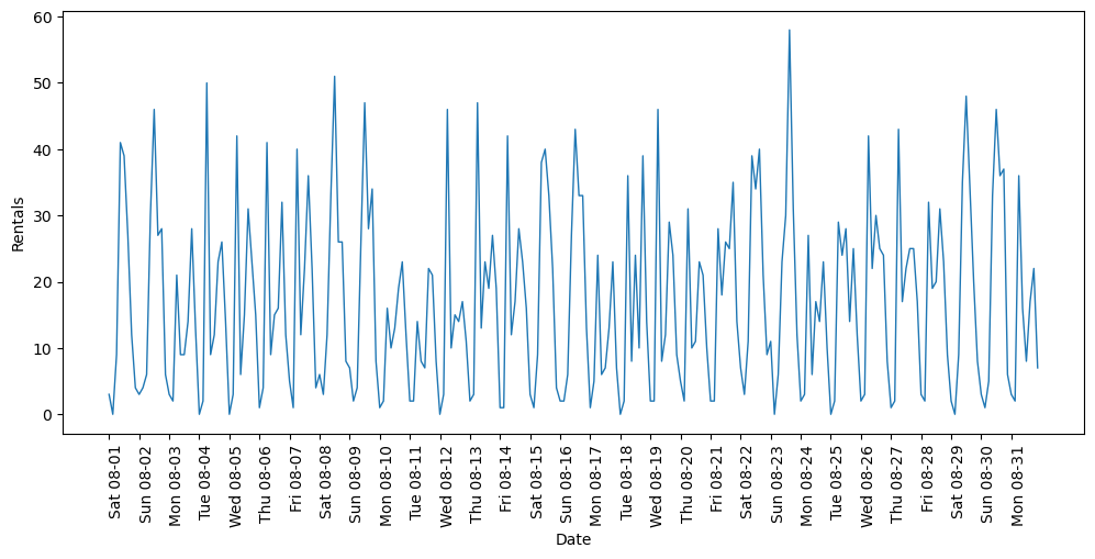
# extract the target values (number of rentals)
y = citibike.values

# convert the time to posixtime (number of seconds that have elapsed
# since the Unix epoch, that is the time 00:00:00 UTC on 1 January 1970):
X = np.array(citibike.index.astype("int")).reshape(-1, 1)
X.shape
(248, 1)from sklearn.linear_model import LinearRegression
from sklearn.ensemble import RandomForestRegressor# use the first 184 data points for training, the rest for testing
n_train = 184
# function to evaluate and plot a regressor on a given feature set
def eval_on_features(features, target, regressor):
# split the given features into a training and test set
X_train, X_test = features[:n_train], features[n_train:]
# split also the
y_train, y_test = target[:n_train], target[n_train:]
regressor.fit(X_train, y_train)
print(f"Test-set R^2: {regressor.score(X_test, y_test):.2f}")
y_pred = regressor.predict(X_test)
y_pred_train = regressor.predict(X_train)
plt.figure(figsize=(12, 5))
plt.xticks(range(0, len(X), 8), my_xticks.strftime("%a %m-%d"), rotation=90, ha="left")
plt.plot(range(n_train), y_train, label="train")
plt.plot(range(n_train, len(y_test) + n_train), y_test, '-', label="test")
plt.plot(range(n_train), y_pred_train, '--', label="prediction train")
plt.plot(range(n_train, len(y_test) + n_train), y_pred, '--', label="prediction test")
plt.legend(loc=(1.01, 0))
plt.xlabel("Date")
plt.ylabel("Rentals")RF_regressor = RandomForestRegressor(n_estimators=100, random_state=0)
eval_on_features(X, y, RF_regressor)Test-set R^2: -0.04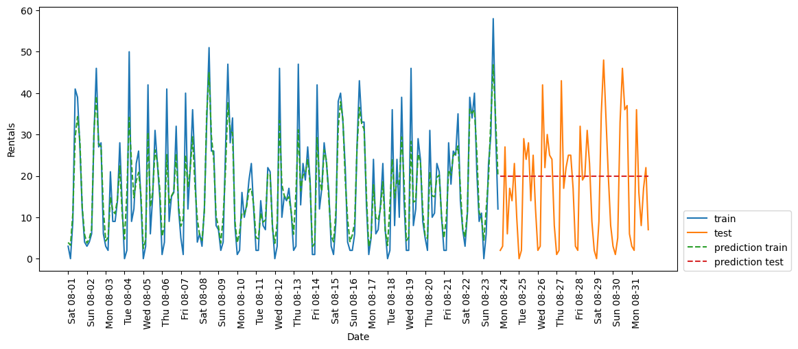
X_hour = np.array(citibike.index.hour).reshape(-1, 1)

eval_on_features(X_hour, y, RF_regressor)
Test-set R^2: 0.60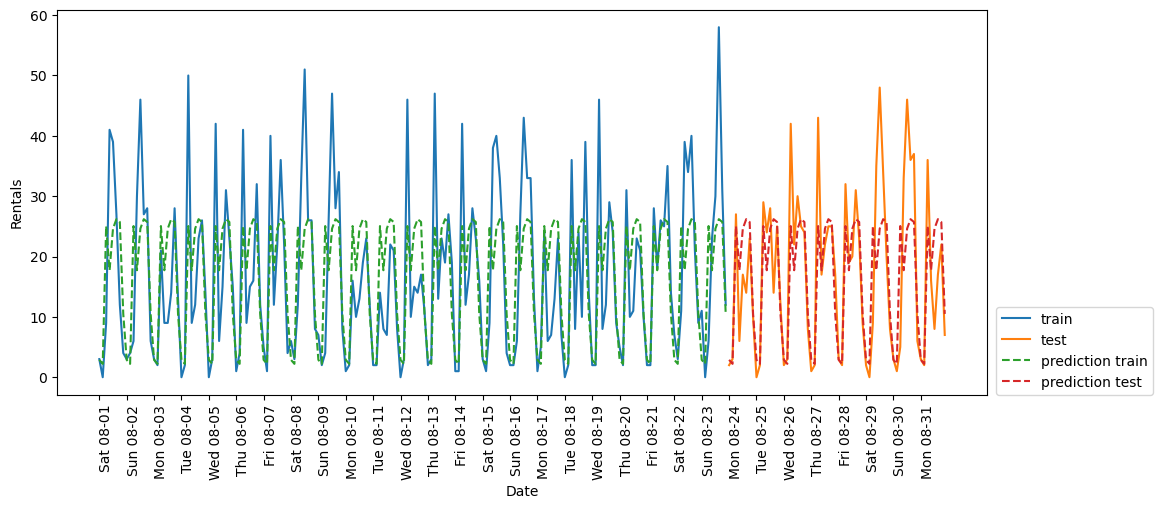
X_hour_week = np.hstack( [ np.array(citibike.index.dayofweek).reshape(-1, 1),
                           np.array(citibike.index.hour).reshape(-1, 1)
                         ] )
print(X_hour_week.shape)

eval_on_features(X_hour_week, y, RF_regressor)
(248, 2)
Test-set R^2: 0.84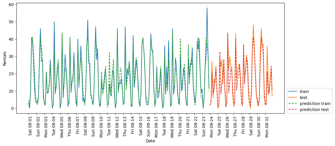
eval_on_features(X_hour_week, y, LinearRegression())Test-set R^2: 0.13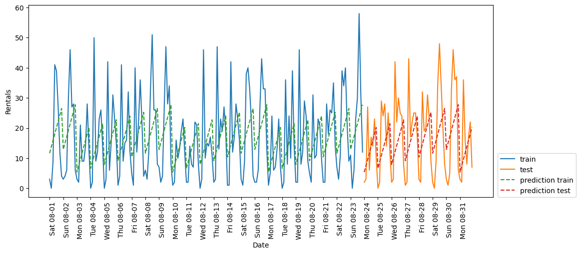
enc = OneHotEncoder(categories='auto')
X_hour_week_onehot = enc.fit_transform(X_hour_week).toarray()
print(X_hour_week_onehot.shape)
print(enc.get_feature_names_out())

eval_on_features(X_hour_week_onehot, y, Ridge())
(248, 15)
['x0_0' 'x0_1' 'x0_2' 'x0_3' 'x0_4' 'x0_5' 'x0_6' 'x1_0' 'x1_3' 'x1_6'
'x1_9' 'x1_12' 'x1_15' 'x1_18' 'x1_21']
Test-set R^2: 0.62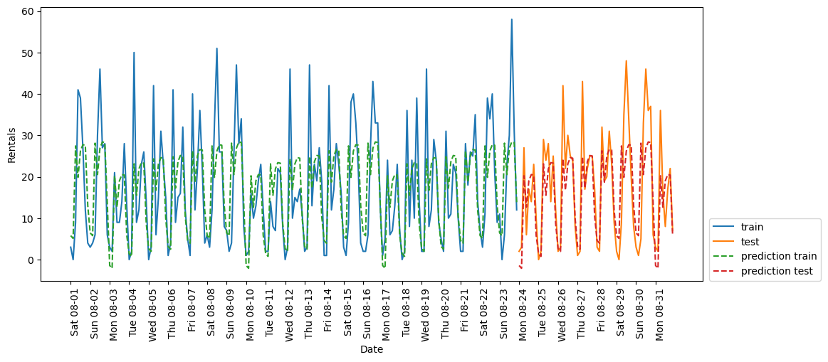
poly_transformer = PolynomialFeatures(degree=2, interaction_only=True,
                                      include_bias=False)
X_hour_week_onehot_poly = poly_transformer.fit_transform(X_hour_week_onehot)
print(X_hour_week_onehot_poly.shape) # 15*14/2 + 15
# print(poly_transformer.get_feature_names_out())

lr = Ridge()
eval_on_features(X_hour_week_onehot_poly, y, lr)
(248, 120)
Test-set R^2: 0.85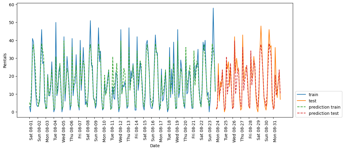
hour = [f"{i:02d}:00" for i in range(0, 24, 3)]
day  = ["Mon", "Tue", "Wed", "Thu", "Fri", "Sat", "Sun"]
features =  day + hour

features_poly    = poly_transformer.get_feature_names_out(features)
features_nonzero = np.array(features_poly)[lr.coef_ != 0]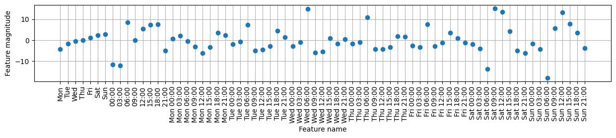
coef_nonzero = lr.coef_[lr.coef_ != 0]plt.figure(figsize=(15, 2))
plt.plot(coef_nonzero, 'o')
plt.xticks(np.arange(len(coef_nonzero)), features_nonzero, rotation=90)
plt.xlabel("Feature name")
plt.ylabel("Feature magnitude")
plt.grid(True)