import pandas as pd
import matplotlib.pyplot as plt
import numpy as np
import mglearn
import seaborn as snsÜbung 3
Decision Trees, Dummy Features, Zeitreihenanalyse, PCA
Python
from sklearn.datasets import load_iris

from sklearn.model_selection import train_test_split

from sklearn.neighbors import KNeighborsRegressor
from sklearn.linear_model import LinearRegression
from sklearn.linear_model import Ridge
from sklearn.linear_model import Lasso
from sklearn.linear_model import LogisticRegression
from sklearn.svm          import LinearSVC
from sklearn.cluster  import KMeans

from scipy.cluster.hierarchy import dendrogram, ward
# set default values for all plotting:
size=12
plt.rcParams['axes.labelsize'] = size
plt.rcParams['xtick.labelsize'] = size
plt.rcParams['ytick.labelsize'] = size
plt.rcParams['legend.fontsize'] = size
plt.rcParams['figure.figsize'] = (6.29, 6/10*6.29)
plt.rcParams['lines.linewidth'] = 1
plt.rcParams['axes.grid'] = True
# print(plt.rcParams)
# import locale #should you want german notation for numbers, then use the locale package
# locale.setlocale(locale.LC_ALL, "deu_deu")
# plt.rcParams['axes.formatter.use_locale'] = True
# Stylefile
# plt.style.use('C:/Users/edel/Documents/Python Scripts/Stylefile/custom_figure_style.mplstyle')Decision Trees
Übung 1: Hotel-Reservations Datensatz mit Forest Classifiern
- Laden Sie den Hotel Reservations Datensatz von Kaggle herunter.
- Betrachten Sie den Datensatz und ersetzen Sie nicht-numerische Features durch Dummy-Features.
- Ermitteln Sie die vier wichtigsten Features des Datensatzes anhand der Korrelationsmatrix und erstellen Sie sinnhafte Darstellungen zwischen dem jeweiligen Feature und dem Target.
- Verwenden Sie den Datensatz und untersuchen Sie die Performance der Ensembles of Decision Tree Algorithmen für unterschiedliche Parameter bei einem fixen Train-Test-Split (random_state=10).
- Erstellen Sie einen Subplot, der 3 Diagramme im Format 3x1 enthält. Plotten Sie jeweils den Testscore in Abhängigkeit des Hyperparameters (max_depth, n_estimators, learning_rate) für die drei untersuchten Algorithmen.
Lösung:
from sklearn.tree import DecisionTreeClassifier
from sklearn.ensemble import RandomForestClassifier
from sklearn.ensemble import GradientBoostingClassifier

df_hotel=pd.read_csv('daten/Hotel Reservations.csv')
df_hotel=df_hotel.drop(columns=['Booking_ID'])
df_h_dummified=pd.get_dummies(df_hotel)
X=df_h_dummified.drop(columns=['booking_status_Canceled','booking_status_Not_Canceled'])
y=df_h_dummified['booking_status_Canceled']
corrs=df_h_dummified.corr().booking_status_Canceled
corrs=abs(corrs)
corrs_sorted=corrs.sort_values(ascending=False)
#print(corrs_sorted)
X_hc=df_h_dummified[['lead_time','arrival_year','avg_price_per_room','no_of_special_requests','booking_status_Canceled']] #highly correlated featuresX_hc.columns=['LT','Year','Price','Specialties','Canceled']
sm=pd.plotting.scatter_matrix(X_hc[::20],
figsize=(15, 12), marker='.',
hist_kwds={'bins': 30,'color':'grey'}, s=30, alpha=.8,color='red',
cmap=plt.get_cmap('coolwarm'))
#y ticklabels
[plt.setp(item.yaxis.get_majorticklabels(), 'size', 14) for item in sm.ravel()]
#x ticklabels
[plt.setp(item.xaxis.get_majorticklabels(), 'size', 14,'rotation',0) for item in sm.ravel()]
#y labels
[plt.setp(item.yaxis.get_label(), 'size', 14, 'rotation',0,'ha','right') for item in sm.ravel()]
#x labels
[plt.setp(item.xaxis.get_label(), 'size',14) for item in sm.ravel()]
plt.tight_layout()
plt.grid(False)/usr/lib/python3.10/site-packages/pandas/plotting/_matplotlib/misc.py:97: UserWarning: No data for colormapping provided via 'c'. Parameters 'cmap' will be ignored
ax.scatter(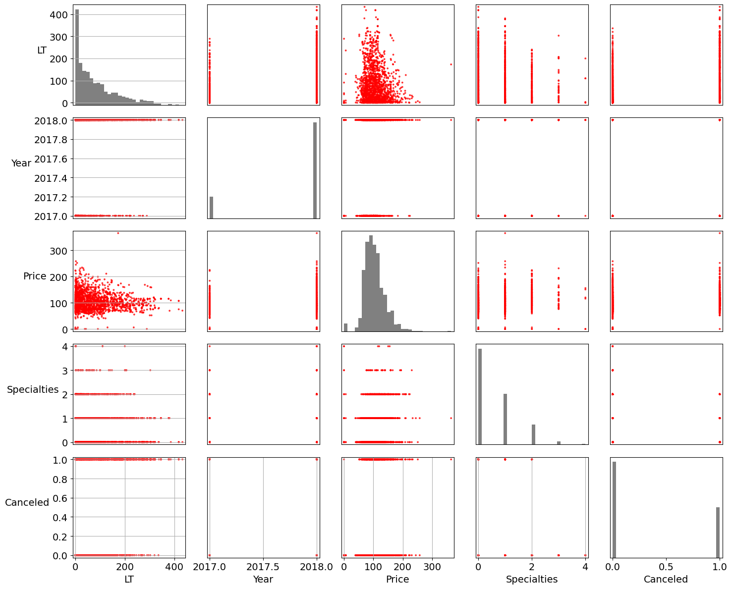
plt.figure()
sns.kdeplot(X_hc.LT[X_hc.Canceled==1],color='black',fill=True,alpha=.2,label='Canceled')
sns.kdeplot(X_hc.LT[X_hc.Canceled==0],color='red',fill=True,alpha=.2,label='Not Canceled')
plt.tight_layout()
plt.xlabel('Tage Buchung vor Reiseantritt')
plt.ylabel('Häufigkeit')
plt.legend()
plt.grid(False)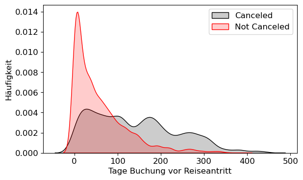
plt.figure()
sns.kdeplot(X_hc.Year[X_hc.Canceled==1],color='black',fill=True,alpha=.2,label='Canceled')
sns.kdeplot(X_hc.Year[X_hc.Canceled==0],color='red',fill=True,alpha=.2,label='Not Canceled')
plt.xticks([2017,2018])
plt.tight_layout()
plt.xlabel('Jahr')
plt.ylabel('Häufigkeit')
plt.yticks(np.arange(0,10.01,2))
plt.legend(loc=2)
plt.grid(False)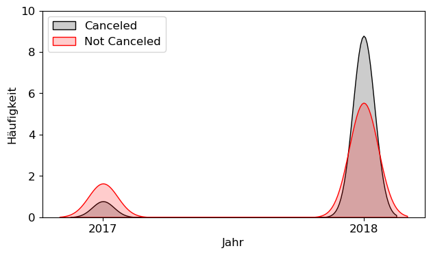
plt.figure()
sns.kdeplot(X_hc.Price[X_hc.Canceled==1],color='black',fill=True,alpha=.2,label='Canceled')
sns.kdeplot(X_hc.Price[X_hc.Canceled==0],color='red',fill=True,alpha=.2,label='Not Canceled')
plt.tight_layout()
plt.xlabel('Preis')
plt.ylabel('Häufigkeit')
plt.legend()
plt.grid(False)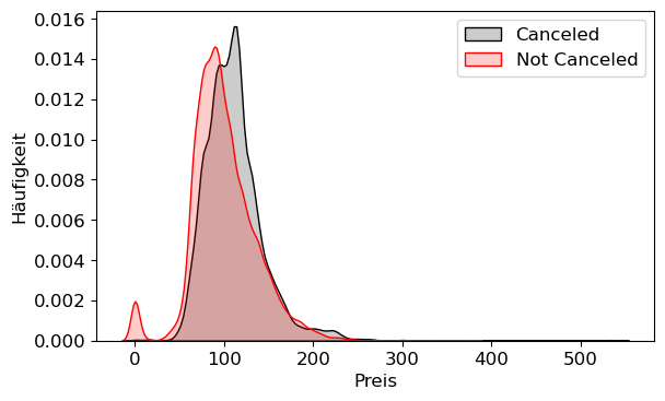
plt.figure()
sns.kdeplot(X_hc.Specialties[X_hc.Canceled==1],color='black',fill=True,alpha=.2,label='Canceled')
sns.kdeplot(X_hc.Specialties[X_hc.Canceled==0],color='red',fill=True,alpha=.2,label='Not Canceled')
plt.tight_layout()
plt.xlabel('Anzahl Sonderwünsche')
plt.ylabel('Häufigkeit')
plt.legend()
plt.grid(False)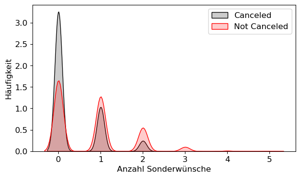
X_train, X_test, y_train, y_test = train_test_split(
    X, y, random_state=10)
#Untersuchen der Performance
algo = DecisionTreeClassifier(max_depth=3)
#algo = RandomForestClassifier(n_estimators=5, random_state=2)
#algo = GradientBoostingClassifier(learning_rate=0.001)
algo.fit(X_train, y_train)
print(f"Accuracy on training set: {algo.score(X_train, y_train):.3f}")
print(f"Accuracy on test set: {algo.score(X_test, y_test):.3f}")Accuracy on training set: 0.786
Accuracy on test set: 0.787# Berechnung der einzelnen Test Scores
DT_string='max_depth'
RF_string='n_estimators'
GB_string='learning_rate'
m_d=np.arange(1,20,1)
n_est=np.arange(1,32,2)
l_r=np.logspace(-3,3,7)
def param_var(algo,DT_stringparam,param):
test_scores=[]
for i in range(len(param)):
params={DT_string:m_d[i]}
algo.set_params(**params)
algo.fit(X_train,y_train)
test_scores.append(algo.score(X_test,y_test))
return test_scores
test_scores_dt=param_var(DecisionTreeClassifier(),DT_string,m_d)
test_scores_rf=param_var(RandomForestClassifier(),RF_string,n_est)
test_scores_gb=param_var(GradientBoostingClassifier(random_state=2),GB_string,l_r)fig=plt.figure(figsize=(6.29,1.8*6.29))
ax1=fig.add_subplot(3,1,1)
ax2=fig.add_subplot(3,1,2)
ax3=fig.add_subplot(3,1,3)
ax1.plot(m_d,test_scores_dt,ls='solid',marker='o',color='black',label='Decision Tree')
ax1.set_xlabel('Max depth')
ax1.set_ylabel('Testscore')
ax1.set_ylim(0,1)
ax1.set_xticks(np.arange(0,20.1,2))
ax1.grid(True)
ax1.legend(loc=4)
ax2.plot(n_est,test_scores_rf,ls='solid',marker='o',color='black',label='Random Forest')
ax2.set_xlabel('Number of estimators')
ax2.set_ylabel('Testscore')
ax2.set_ylim(0,1)
ax2.grid(True)
ax2.legend(loc=4)
ax3.semilogx(l_r,test_scores_gb,ls='solid',marker='o',color='black',label='Gradient Boosting')
ax3.set_xlabel('Learning rate')
ax3.set_ylabel('Testscore')
ax3.set_ylim(0,1)
ax3.grid(True)
ax3.legend(loc=4)
fig.tight_layout()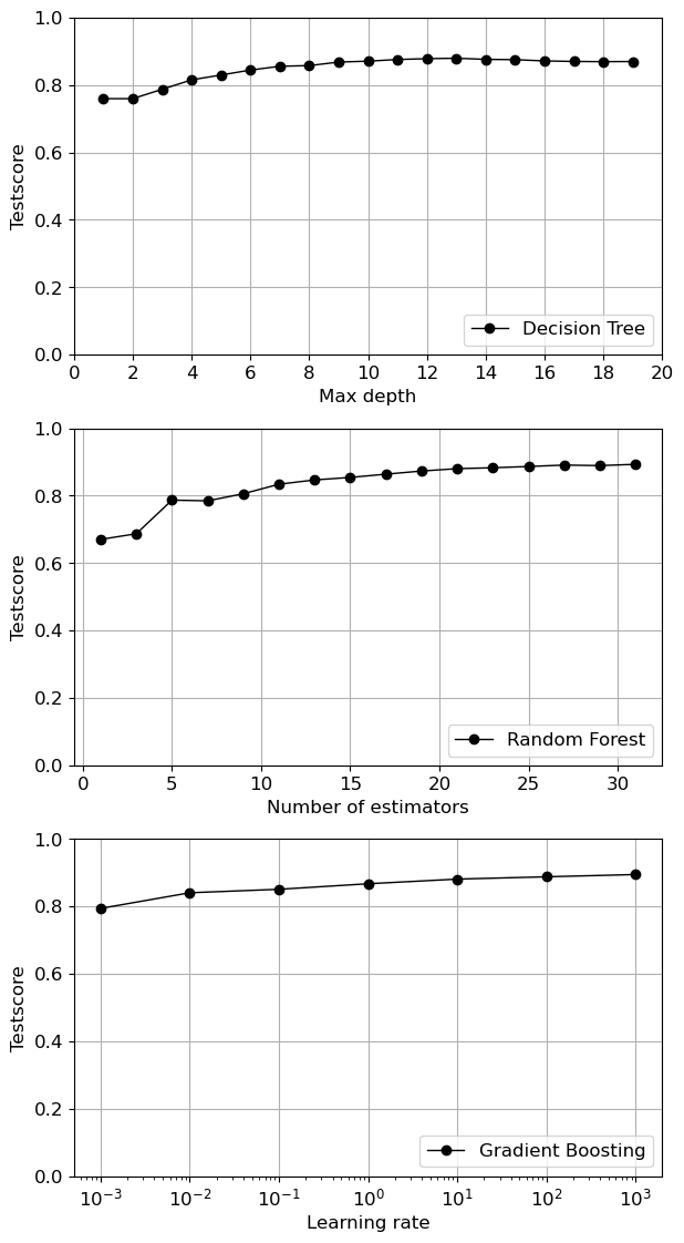
Aufgabe 1: 24h-Strompreise
Untersuchen Sie die 24h-Strompreise der Datei dshistory2017.xls der EXAA (Energy Exchange Austria bzgl. der Frage: “Wie gut kann man aus der Uhrzeit (Stunde 1, 2, …, 24) und dem Wochentag (Mo, Di, …) vorhersagen, ob der Strompreis Price (EUR) über oder unter dem Tagesmittel liegt?”
- Machen Sie sich zuerst passende Abbildungen der Daten.
- Bringen Sie die Daten in die übliche \(X\)-\(y\)-Form.
- Vergleichen Sie verschiedene Algorithmen.
Lösung:
price = pd.read_excel('daten/dshistory2017.xls', sheet_name='Price (EUR)',
                      index_col=0, skiprows=1)
df = price.iloc[:,:24].copy()
df.shape
# check=df.applymap(np.isreal)
#print(df.dtypes)
df=df[df.applymap(np.isreal).all('columns')] #Only if all columns in a row are real values the row is not dropped
df.dropna(inplace=True) #dropNANs
print(df.shape)
(363, 24)df.head(3)| hEXA01 | hEXA02 | hEXA03 | hEXA04 | hEXA05 | hEXA06 | hEXA07 | hEXA08 | hEXA09 | hEXA10 | ... | hEXA15 | hEXA16 | hEXA17 | hEXA18 | hEXA19 | hEXA20 | hEXA21 | hEXA22 | hEXA23 | hEXA24 | |
|---|---|---|---|---|---|---|---|---|---|---|---|---|---|---|---|---|---|---|---|---|---|
| Delivery Date | |||||||||||||||||||||
| 2017-12-31 | -20.1 | -28.2 | -38.78 | -25.63 | -17.60 | -19.93 | -27.88 | -17.35 | -4.99 | 1.41 | ... | -36.82 | -20.78 | 3.02 | 14.18 | 13.28 | 7.34 | 0.04 | 1.91 | 10.05 | 5.53 |
| 2017-12-30 | 15.5 | 10.7 | 8.20 | 8.20 | 9.40 | 10.30 | 8.81 | 10.99 | 17.49 | 23.22 | ... | 16.00 | 14.90 | 15.54 | 18.71 | 17.00 | 14.31 | 6.78 | 1.69 | 0.55 | -6.87 |
| 2017-12-29 | 7.2 | 4.89 | 3.56 | 3.23 | 3.84 | 9.13 | 15.32 | 26.06 | 30.99 | 32.22 | ... | 31.20 | 34.60 | 38.96 | 40.54 | 38.20 | 34.12 | 30.58 | 28.80 | 28.61 | 19.86 |
3 rows × 24 columns
# Maximale Tageswerte:
plt.figure()
plt.plot(df.max(axis=1),color='red')
plt.ylim(0,150)
plt.xlabel('Datum (YYYY-MM)')
plt.ylabel('Preis (€/MWh)')
plt.tight_layout()

print(df.max(axis=1).max())
143.1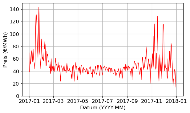
Falschfarbenbild der Rohdaten, colormaps
X = np.array([[1,2],
              [3,4],
              [5,6]])
plt.imshow(X, cmap=plt.cm.YlOrRd, extent=[0, 24, 0, 36.3], aspect='auto')
plt.colorbar();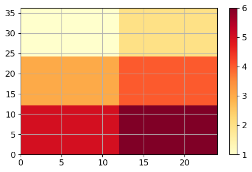
Z = df.values.astype(float)plt.figure()
plt.imshow(Z, interpolation='bilinear', # compare with interpolation=None
cmap=plt.cm.coolwarm, extent=[0, 24, 0, 363], aspect='auto');
plt.xlabel('Stunde')
plt.ylabel('Tag')
plt.colorbar()
plt.grid(False);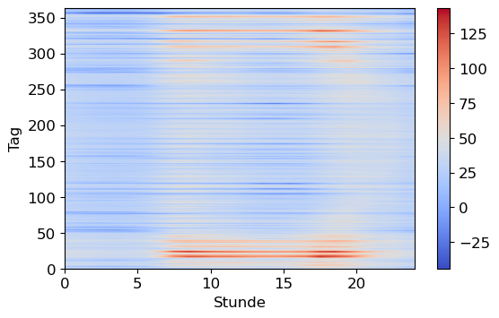
df['mean'] = df.apply(np.mean, axis=1) #Mittelwerte
df['day']  = df.index.dayofweek    # Monday=0, Sunday=6
df.head(3)| hEXA01 | hEXA02 | hEXA03 | hEXA04 | hEXA05 | hEXA06 | hEXA07 | hEXA08 | hEXA09 | hEXA10 | ... | hEXA17 | hEXA18 | hEXA19 | hEXA20 | hEXA21 | hEXA22 | hEXA23 | hEXA24 | mean | day | |
|---|---|---|---|---|---|---|---|---|---|---|---|---|---|---|---|---|---|---|---|---|---|
| Delivery Date | |||||||||||||||||||||
| 2017-12-31 | -20.1 | -28.2 | -38.78 | -25.63 | -17.60 | -19.93 | -27.88 | -17.35 | -4.99 | 1.41 | ... | 3.02 | 14.18 | 13.28 | 7.34 | 0.04 | 1.91 | 10.05 | 5.53 | -12.000833 | 6 |
| 2017-12-30 | 15.5 | 10.7 | 8.20 | 8.20 | 9.40 | 10.30 | 8.81 | 10.99 | 17.49 | 23.22 | ... | 15.54 | 18.71 | 17.00 | 14.31 | 6.78 | 1.69 | 0.55 | -6.87 | 13.447917 | 5 |
| 2017-12-29 | 7.2 | 4.89 | 3.56 | 3.23 | 3.84 | 9.13 | 15.32 | 26.06 | 30.99 | 32.22 | ... | 38.96 | 40.54 | 38.20 | 34.12 | 30.58 | 28.80 | 28.61 | 19.86 | 24.196667 | 4 |
3 rows × 26 columns
# binäre Abweichung vom Tagesmittel:
for h in range(1, 25):
    df[h] = df.iloc[:,h-1] - df['mean']
#     for i in range(len(df['mean'])):
#         if df.iloc[i,h+25]>0:
#             df.iloc[i,h+25]=1
#         else:
#             df.iloc[i,h+25]=0
df[h] = df[h].apply(lambda x: 1 if x > 0 else 0)df.head(3)| hEXA01 | hEXA02 | hEXA03 | hEXA04 | hEXA05 | hEXA06 | hEXA07 | hEXA08 | hEXA09 | hEXA10 | ... | 15 | 16 | 17 | 18 | 19 | 20 | 21 | 22 | 23 | 24 | |
|---|---|---|---|---|---|---|---|---|---|---|---|---|---|---|---|---|---|---|---|---|---|
| Delivery Date | |||||||||||||||||||||
| 2017-12-31 | -20.1 | -28.2 | -38.78 | -25.63 | -17.60 | -19.93 | -27.88 | -17.35 | -4.99 | 1.41 | ... | 0 | 0 | 1 | 1 | 1 | 1 | 1 | 1 | 1 | 1 |
| 2017-12-30 | 15.5 | 10.7 | 8.20 | 8.20 | 9.40 | 10.30 | 8.81 | 10.99 | 17.49 | 23.22 | ... | 1 | 1 | 1 | 1 | 1 | 1 | 0 | 0 | 0 | 0 |
| 2017-12-29 | 7.2 | 4.89 | 3.56 | 3.23 | 3.84 | 9.13 | 15.32 | 26.06 | 30.99 | 32.22 | ... | 1 | 1 | 1 | 1 | 1 | 1 | 1 | 1 | 1 | 0 |
3 rows × 50 columns
my_df = df.melt(id_vars=['day'], value_vars=range(1,25))
display(my_df.head(3))
display(my_df.tail(3))| day | variable | value | |
|---|---|---|---|
| 0 | 6 | 1 | 0 |
| 1 | 5 | 1 | 1 |
| 2 | 4 | 1 | 0 |
| day | variable | value | |
|---|---|---|---|
| 8709 | 1 | 24 | 0 |
| 8710 | 0 | 24 | 0 |
| 8711 | 6 | 24 | 0 |
my_df.rename(columns={"variable":"hour", "value":"above"}, inplace=True)
my_df.head(3)| day | hour | above | |
|---|---|---|---|
| 0 | 6 | 1 | 0 |
| 1 | 5 | 1 | 1 |
| 2 | 4 | 1 | 0 |
my_pred = pd.pivot_table(my_df, index='day', columns='hour',
                         values='above', aggfunc=np.mean)
my_pred.sort_index(ascending=False, inplace=True)
my_pred| hour | 1 | 2 | 3 | 4 | 5 | 6 | 7 | 8 | 9 | 10 | ... | 15 | 16 | 17 | 18 | 19 | 20 | 21 | 22 | 23 | 24 |
|---|---|---|---|---|---|---|---|---|---|---|---|---|---|---|---|---|---|---|---|---|---|
| day | |||||||||||||||||||||
| 6 | 0.627451 | 0.411765 | 0.176471 | 0.098039 | 0.137255 | 0.098039 | 0.078431 | 0.156863 | 0.333333 | 0.411765 | ... | 0.176471 | 0.215686 | 0.411765 | 0.666667 | 1.000000 | 1.000000 | 0.980392 | 0.901961 | 0.921569 | 0.607843 |
| 5 | 0.519231 | 0.269231 | 0.192308 | 0.173077 | 0.115385 | 0.134615 | 0.115385 | 0.423077 | 0.846154 | 0.923077 | ... | 0.134615 | 0.250000 | 0.365385 | 0.750000 | 1.000000 | 0.980769 | 0.788462 | 0.634615 | 0.634615 | 0.423077 |
| 4 | 0.076923 | 0.019231 | 0.000000 | 0.000000 | 0.000000 | 0.038462 | 0.538462 | 1.000000 | 1.000000 | 1.000000 | ... | 0.326923 | 0.384615 | 0.480769 | 0.846154 | 1.000000 | 0.980769 | 0.846154 | 0.615385 | 0.538462 | 0.192308 |
| 3 | 0.076923 | 0.038462 | 0.019231 | 0.019231 | 0.019231 | 0.000000 | 0.576923 | 0.980769 | 1.000000 | 0.980769 | ... | 0.365385 | 0.442308 | 0.538462 | 0.903846 | 0.980769 | 1.000000 | 0.769231 | 0.673077 | 0.519231 | 0.173077 |
| 2 | 0.076923 | 0.000000 | 0.000000 | 0.000000 | 0.000000 | 0.000000 | 0.576923 | 1.000000 | 1.000000 | 1.000000 | ... | 0.326923 | 0.365385 | 0.461538 | 0.903846 | 0.961538 | 0.961538 | 0.903846 | 0.576923 | 0.423077 | 0.115385 |
| 1 | 0.019231 | 0.000000 | 0.000000 | 0.000000 | 0.000000 | 0.000000 | 0.557692 | 0.961538 | 0.980769 | 0.961538 | ... | 0.365385 | 0.384615 | 0.480769 | 0.903846 | 1.000000 | 0.980769 | 0.826923 | 0.692308 | 0.519231 | 0.096154 |
| 0 | 0.038462 | 0.019231 | 0.019231 | 0.019231 | 0.019231 | 0.019231 | 0.653846 | 0.942308 | 0.903846 | 0.942308 | ... | 0.403846 | 0.480769 | 0.634615 | 0.923077 | 1.000000 | 1.000000 | 0.961538 | 0.788462 | 0.615385 | 0.134615 |
7 rows × 24 columns
plt.figure()
plt.imshow(my_pred.values, cmap=plt.cm.bwr, extent=[0, 24, 0, 6],
           aspect='auto', interpolation='bilinear') # compare with interpolation=None
plt.xlabel('hour')
plt.ylabel('day')
plt.colorbar();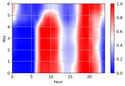
X = my_df[['hour','day']].values
X
array([[1, 6],
[1, 5],
[1, 4],
...,
[24, 1],
[24, 0],
[24, 6]], dtype=object)y = my_df['above'].values
yarray([0, 1, 0, ..., 0, 0, 0])X_train, X_test, y_train, y_test = train_test_split(X, y, random_state=10)algo = DecisionTreeClassifier(max_depth=3)
algo = RandomForestClassifier(n_estimators=5, random_state=0)
algo = GradientBoostingClassifier(learning_rate=0.1, n_estimators=35)
algo.fit(X_train, y_train)
print(f"Accuracy on training set: {algo.score(X_train, y_train):.3f}")
print(f"Accuracy on test set: {algo.score(X_test, y_test):.3f}")Accuracy on training set: 0.809
Accuracy on test set: 0.811def plot_tree_partition(X, y, tree):
eps = 0.5
x_min, x_max = X[:, 0].min() - eps, X[:, 0].max() + eps
y_min, y_max = X[:, 1].min() - eps, X[:, 1].max() + eps
xx = np.linspace(x_min, x_max, 1000)
yy = np.linspace(y_min, y_max, 1000)
X1, X2 = np.meshgrid(xx, yy)
X_grid = np.column_stack((X1.ravel(), X2.ravel()))
Z = tree.predict(X_grid)
Z = Z.reshape(X1.shape)
plt.contourf(X1, X2, Z, alpha=.4, levels=[0, .5, 1])
# mglearn.discrete_scatter(X[:, 0], X[:, 1], y, alpha=0.1)
returnplt.figure()
plot_tree_partition(X, y, algo)
plt.xlabel('hour')
plt.ylabel('day')
plt.grid(True);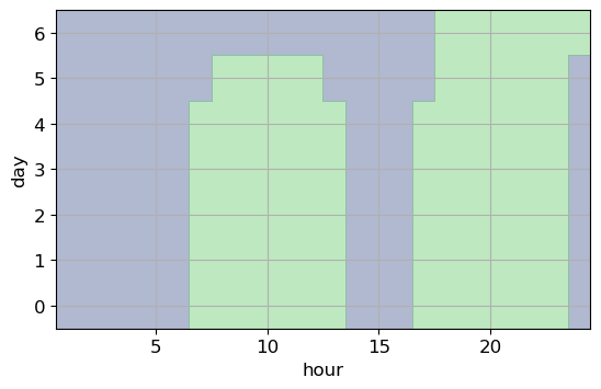
Principal Component Analysis
Übung 2: Prognose mit/ohne Feature Reduktion
Laden Sie die Datei ETW.xlsx in ein pandas DataFrame.
- Erstellen Sie einen Scatter-Matrix-Plot der Daten.
- Stellen Sie das Target
AMin Abhängigkeit des FeaturesMathematikin einer Scatter-Matrix dar. Fitten Sie eine Gerade durch die Datenpunkte. - Berechnen Sie alle Korrelationen.
- Erstellen und bewerten Sie mehrere Modelle zur Prognose der Spalte
AMaus den anderen Spalten. - Verwenden Sie PCA zur Prognose der Spalte
AMaus den ersten zwei Hauptkomponenten. Stellen Sie die Ergebnisse grafisch dar.
Lösung:
df = pd.read_excel("daten/ETW.xlsx", index_col=0)
df.head(3)| Interview | Mathematik | Physik | Chemie | AM | |
|---|---|---|---|---|---|
| 0 | 0.860 | 0.391304 | 0.500000 | 0.6000 | 58.750 |
| 1 | 0.885 | 0.586957 | 0.095238 | 0.1250 | 57.600 |
| 2 | 0.750 | 0.739130 | 0.714286 | 0.3875 | 63.705 |
sm=pd.plotting.scatter_matrix(df,
                           figsize=(15, 12), marker='.', diagonal='kde', density_kwds={'color':'black'},
                           s=30, alpha=.8,color='red',
                           cmap=plt.get_cmap('coolwarm'))

#y ticklabels
[plt.setp(item.yaxis.get_majorticklabels(), 'size', 14) for item in sm.ravel()]
#x ticklabels
[plt.setp(item.xaxis.get_majorticklabels(), 'size', 14,'rotation',0) for item in sm.ravel()]
#y labels
[plt.setp(item.yaxis.get_label(), 'size', 14, 'rotation',0,'ha','right') for item in sm.ravel()]
#x labels
[plt.setp(item.xaxis.get_label(), 'size',14) for item in sm.ravel()]

plt.tight_layout()
plt.grid(False)
/usr/lib/python3.10/site-packages/pandas/plotting/_matplotlib/misc.py:97: UserWarning: No data for colormapping provided via 'c'. Parameters 'cmap' will be ignored
ax.scatter(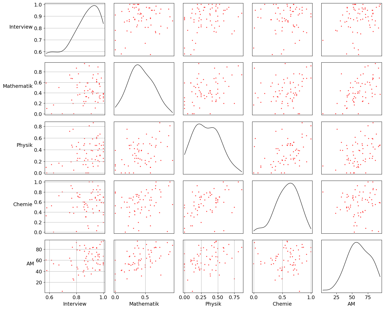
coefs=np.polyfit(df.Mathematik*100,df.AM,1)
t=np.arange(0,100.1,1)
y=coefs[0]*t+coefs[1]

plt.figure()
plt.scatter(df.Mathematik*100,df.AM,color='red')
plt.plot(t,y,lw=2,ls='solid',color='black')
plt.xlabel('Mathematik Aufnahmetest (%)')
plt.ylabel('Angewandte Mathematik Prüfung (%)')
plt.ylim(0,100)
plt.yticks(np.arange(0,100.1,20))
plt.tight_layout()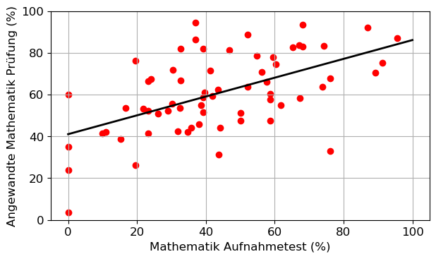
df.corr()| Interview | Mathematik | Physik | Chemie | AM | |
|---|---|---|---|---|---|
| Interview | 1.000000 | 0.162706 | 0.314272 | 0.107939 | 0.271260 |
| Mathematik | 0.162706 | 1.000000 | 0.360859 | 0.231434 | 0.552820 |
| Physik | 0.314272 | 0.360859 | 1.000000 | 0.434040 | 0.336828 |
| Chemie | 0.107939 | 0.231434 | 0.434040 | 1.000000 | 0.061733 |
| AM | 0.271260 | 0.552820 | 0.336828 | 0.061733 | 1.000000 |
features = ["Interview", "Mathematik", "Physik", "Chemie"]
# features = ["Mathematik", "Physik"]
X = df[features].values
y = df.AM.values
# X_train, X_test, y_train, y_test = train_test_split(X, y, random_state=None)
X_train, X_test, y_train, y_test = train_test_split(X, y, random_state=0)
algo = KNeighborsRegressor(n_neighbors=10)
algo = LinearRegression()
# algo = Ridge(alpha=.1)
# algo = Lasso(alpha=.25)
algo.fit(X_train, y_train)
print("train score: {:.2f}".format(algo.score(X_train, y_train)))
print("test score: {:.2f}".format(algo.score(X_test, y_test)))train score: 0.35
test score: 0.31algo.intercept_31.491830606311968algo.coef_array([ 15.34341359, 39.10870341, 18.66945353, -14.64473302])plt.figure(figsize=(8,5))
plt.stem(np.concatenate( ([algo.intercept_], algo.coef_) ))
plt.xlabel('feature')
plt.xticks(range(len(features) + 1), ['intercept'] + features)
plt.ylabel('regression coefficient')
plt.grid(True)
from sklearn.decomposition import PCApca = PCA(n_components=2)
pca.fit(X)
X_pca = pca.transform(X)
print("Original shape: {}".format(str(X.shape)))
print("Reduced shape : {}".format(str(X_pca.shape)))Original shape: (65, 4)
Reduced shape : (65, 2)# plot fist vs second principal component, color by class:
plt.figure(figsize=(7,7))
plt.scatter(X_pca[:, 0], X_pca[:, 1])
plt.xlabel("First principal component")
plt.ylabel("Second principal component")
plt.grid(True)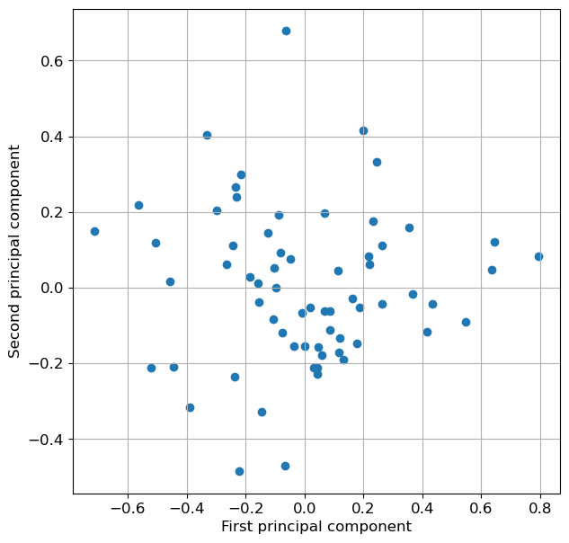
plt.matshow(pca.components_, cmap='viridis')
plt.yticks([0, 1], ["First component", "Second component"])
plt.colorbar()
plt.xticks(range(len(features)), features, rotation=60, ha='left')
plt.xlabel("Feature")
plt.ylabel("Principal components");

pca.components_
array([[ 0.10098801, 0.53178411, 0.55359898, 0.63287854],
[ 0.03665652, 0.77467872, -0.02995449, -0.63058061]])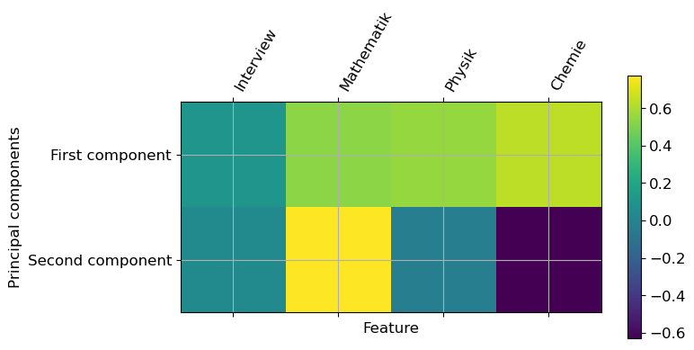
X_train, X_test, y_train, y_test = train_test_split(X_pca, y, random_state=0)

algo = KNeighborsRegressor(n_neighbors=10)
algo = LinearRegression()
#algo = Ridge(alpha=1)
#algo = Lasso(alpha=.5)

algo.fit(X_train, y_train)

print("train score: {:.2f}".format(algo.score(X_train, y_train)))
print("test  score: {:.2f}".format(algo.score(X_test, y_test)))
#algo.coef_
train score: 0.34
test score: 0.28