import pandas as pd
import matplotlib.pyplot as plt
import numpy as np
import seaborn as snsÜbung 1
Beispiele zur Datenverarbeitung und -analyse, erste Klassifizierung und erste Regression
Datenmanagement mit Pandas
Some Links:
- Pandas: Documentation
- Pandas: Getting Started
- Real Python: Using Pandas and Python to Explore Your Dataset
- Python: Date and Time Format Codes
# set default values for all plotting:
size = 12
plt.rcParams['axes.titlesize'] = size
plt.rcParams['axes.labelsize'] = size
plt.rcParams['xtick.labelsize'] = size
plt.rcParams['ytick.labelsize'] = size
plt.rcParams['legend.fontsize'] = size
plt.rcParams['figure.figsize'] = (6.29, 6/10*6.29)
plt.rcParams['lines.linewidth'] = 2
# print(plt.rcParams)

# import locale   # should you want german notation for numbers, then use the locale package
# locale.setlocale(locale.LC_ALL, "deu_deu")
# plt.rcParams['axes.formatter.use_locale'] = True

# Stylefile:
# plt.style.use('custom_figure_style.mplstyle')
Aufgabe 1: Beispielplot für Dokument
t = np.arange(0, 10.01, 0.1)

plt.figure()
plt.plot(t, t**2, color='red', ls='--', label='Polynom 2. Ordnung')
plt.plot(t, t**3, color='black', ls='solid', label='Polynom 3. Ordnung')
plt.annotate('Rotes Polynom', xy=(8, 100), xycoords='data', xytext=(4,600),
             arrowprops=dict(arrowstyle='-|>'), fontsize=size)
plt.xlabel('x-Achse (mm)')
plt.ylabel('y-Achse (mm)')
plt.xlim(0, 10)
plt.ylim(0, 1000)
plt.xticks(np.arange(0, 10.1, 1))
plt.legend()
plt.grid(ls='--', lw=.7)
plt.tight_layout()
plt.savefig('abbildungen/Testplot.jpg', dpi=600)  # relative path
# plt.savefig('C:/Users/edel/Desktop/Testplot.jpg', dpi=600)  # absolute path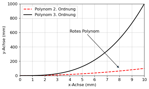
Aufgabe 2: Überlebende der Titanic: Datensatz einlesen, Pre-Processing und Visualisierung
Data Frame: A pandas data frame is a 2-dimensional labeled data structure with columns of potentially different types. Along with the data, a data frame is framed by an index (row labels) and columns (column labels).
Read Data:
- Download the csv-Files
train.csvfrom Kaggle and read the description text. - Read
train.csvinto a pandas data frame first and investigate the data. - Handle non-numeric data accordingly.
- Visualize the data appropriately.
- Let a classification-algorithm train on the data. Make a first classification on the test data and calculate the test score.
df = pd.read_csv("daten/train.csv", index_col='PassengerId')
df.head(3)

# plt.figure()
# sns.heatmap(df.isnull(),cbar=False)

# print(df.columns)
df.drop(columns=['Name', 'Ticket'], inplace=True)
df['Age'].replace(np.NaN, (df['Age'].mean()), inplace=True)  # df.Age = df['Age']
df['Cabin'].replace(np.NaN, 'XXX', inplace=True)
df['Embarked'].replace(np.NaN, 'XXX', inplace=True)
df['Deck'] = df.Cabin.astype(str).str[0]
df.drop(columns='Cabin', inplace=True)

df = pd.get_dummies(df)

df.drop(columns=['Sex_male', 'Embarked_XXX', 'Deck_X'], inplace=True)
plt.figure()
df[df.Survived == 1].Fare.hist(alpha=.5, bins=10, label='Survived')
df[df.Survived == 0].Fare.hist(alpha=.5, bins=10, label='Not Survived')
plt.xlabel('Preis ($)')
plt.ylabel('Anzahl der Passagiere (-)')
plt.legend()
plt.tight_layout()
plt.savefig('abbildungen/Histogram_survived_fare.jpg', dpi=600)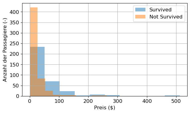
plt.figure()
sns.countplot(x='Pclass', hue='Survived', data=df)
plt.xlabel('Passagierklasse')
plt.yticks(np.arange(0, 501, 50))
plt.tight_layout()
plt.grid(False)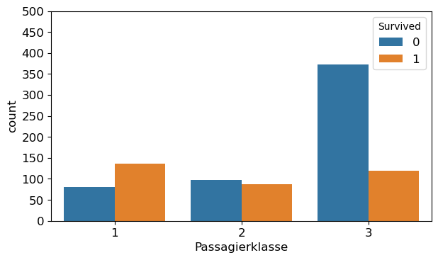
plt.figure()
sns.countplot(x='Sex_female', hue='Survived', data=df)
plt.xlabel('Weiblich')
plt.yticks(np.arange(0, 501, 50))
plt.tight_layout()
plt.grid(False)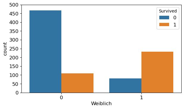
plt.figure()
plt.hist(df.Age, bins=12);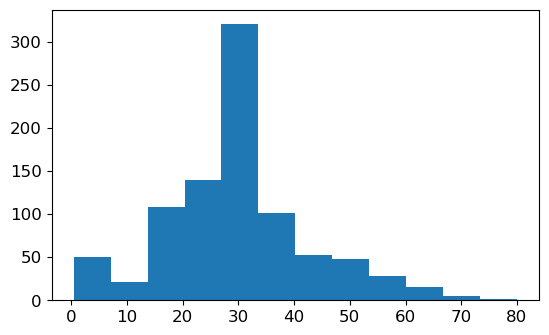
sns.boxplot(data=df, x='Pclass', y='Age');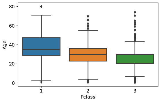
plt.figure()
df2 = df[['Age', 'Fare', 'Pclass', 'Sex_female', 'Survived']]
sm = pd.plotting.scatter_matrix(df2[::3], c=df.Survived[::3], figsize=(12, 12),
                                hist_kwds={'bins': 30, 'color': 'grey'},
                                s=60, alpha=0.8, cmap='coolwarm', ax=None)
for ax in sm.ravel():
    ax.grid(False)

[plt.setp(item.yaxis.get_majorticklabels(), 'size', 14) for item in sm.ravel()]
[plt.setp(item.xaxis.get_majorticklabels(), 'size', 14, 'rotation', 0)
 for item in sm.ravel()]
[plt.setp(item.yaxis.get_label(), 'size', 14, 'rotation', 0, 'ha', 'right')
 for item in sm.ravel()]
[plt.setp(item.xaxis.get_label(), 'size', 14) for item in sm.ravel()]
plt.savefig('abbildungen/Scatter_matrix.png', dpi=600)
<Figure size 629x377.4 with 0 Axes>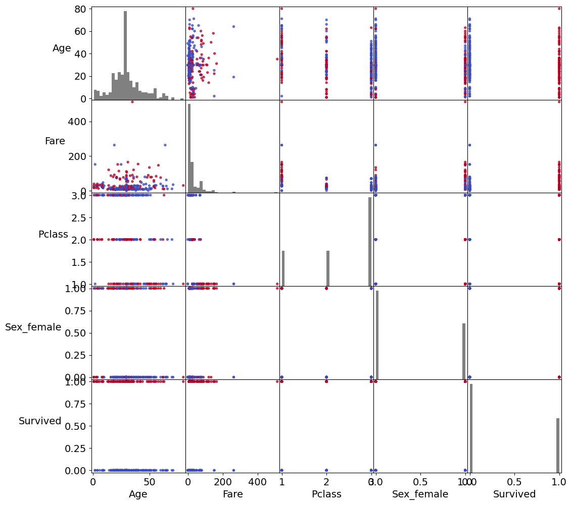
df2.corr()| Age | Fare | Pclass | Sex_female | Survived | |
|---|---|---|---|---|---|
| Age | 1.000000 | 0.091566 | -0.331339 | -0.084153 | -0.069809 |
| Fare | 0.091566 | 1.000000 | -0.549500 | 0.182333 | 0.257307 |
| Pclass | -0.331339 | -0.549500 | 1.000000 | -0.131900 | -0.338481 |
| Sex_female | -0.084153 | 0.182333 | -0.131900 | 1.000000 | 0.543351 |
| Survived | -0.069809 | 0.257307 | -0.338481 | 0.543351 | 1.000000 |
Klassifizierung
X = df.drop(columns='Survived').values  # Features
y = df.Survived.values  # Target

n_splits = 50
n_neighbors = 10
mean_test_scores = []
mean_train_scores = []

from sklearn.model_selection import train_test_split
from sklearn.neighbors import KNeighborsClassifier

for j in range(n_neighbors):
    test_scores = []
    train_scores = []
    for i in range(n_splits):
        X_train, X_test, y_train, y_test = train_test_split(X, y, random_state=i)
        knn = KNeighborsClassifier(n_neighbors=j+1)  # Definition des Algorithmus
        knn.fit(X_train, y_train)   # Trainieren des Algorithmus
        train_scores.append(knn.score(X_train, y_train))
        test_scores.append(knn.score(X_test, y_test))
    mean_test_scores.append(np.mean(test_scores))
    mean_train_scores.append(np.mean(train_scores))

# print(mean_test_scores)
# print(mean_train_scores)
print('Die optimale Anzahl an Nachbarn ist=', np.argmax(mean_test_scores)+1)
Die optimale Anzahl an Nachbarn ist= 7neighbors_arr = np.arange(1, n_neighbors + 1, 1)
# print(neighbors_arr)
plt.figure()
plt.plot(neighbors_arr, mean_test_scores, label='Test Scores')
plt.plot(neighbors_arr, mean_train_scores, label='Train Scores')
plt.ylim(0, 1)
plt.xlim(10, 1)
plt.xticks(np.arange(1, n_neighbors + 1, 1))
plt.xlabel('Anzahl an Nachbarn')
plt.ylabel('Mittlere Scores')
plt.legend(loc=4)
plt.grid(True)
plt.tight_layout()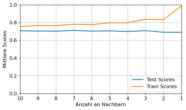
plt.figure()
plt.hist(test_scores, alpha=.5, label='Test Scores')
plt.hist(train_scores, alpha=.5, label='Train Scores')
plt.axvline(x=np.mean(test_scores), color='black')
plt.tight_layout()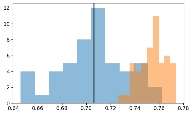
Predictions = knn.predict(X_test)
# print(Predictions)
# print(y_test)

plt.figure()
plt.plot(y_test[::5] - Predictions[::5],
         label='Differenz zwischen Vorhersage und echten Werten',
         ls='none', marker='x')
plt.axhline(y=0, color='black', lw=.5)
plt.legend(loc='best')
plt.ylim(-2, 2)
plt.tight_layout()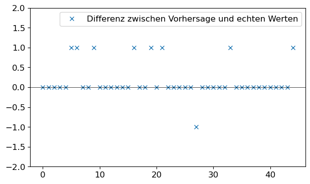
X_train, X_test, y_train, y_test = train_test_split(X, y, random_state=10)
knn = KNeighborsClassifier(n_neighbors=7)  # Definition des Algorithmus
knn.fit(X_train, y_train)
y_pred = knn.predict(X_test)

from sklearn.metrics import confusion_matrix
from sklearn.metrics import ConfusionMatrixDisplay

conf = confusion_matrix(y_test, y_pred)
print(conf)

ConfusionMatrixDisplay(conf).plot()
plt.tight_layout()
[[126 21]
[ 35 41]]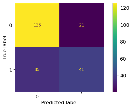
Aufgabe 3: Vorhersagemodell der Kraftwerksleistung
Read Data:
- Download the Data-Files from UCI Machine Learning Repository and read the description text.
- Plot the power output vs. the ambient temperature. Fit a first-order polynome in the data.
- Investigate the data using a scatter matrix.
- Train a regression model to predict the power output and visualize it appropriately.
df_pp = pd.read_excel("daten/CCPP/Folds5x2_pp.xlsx", sheet_name='Sheet1')
df_pp.columns = ['Ambient_Temperature', 'Vacuum', 'Ambient_Pressure',
                 'Relative_Humidity', 'Power_Output']
sns.heatmap(df_pp.isnull(), cbar=False);
df_pp.head()| Ambient_Temperature | Vacuum | Ambient_Pressure | Relative_Humidity | Power_Output | |
|---|---|---|---|---|---|
| 0 | 14.96 | 41.76 | 1024.07 | 73.17 | 463.26 |
| 1 | 25.18 | 62.96 | 1020.04 | 59.08 | 444.37 |
| 2 | 5.11 | 39.40 | 1012.16 | 92.14 | 488.56 |
| 3 | 20.86 | 57.32 | 1010.24 | 76.64 | 446.48 |
| 4 | 10.82 | 37.50 | 1009.23 | 96.62 | 473.90 |
df_pp_sel = df_pp[::20]

# sklearn LinearRegression()

coefs = np.polyfit(df_pp_sel.Ambient_Temperature, df_pp_sel.Power_Output, 1)

T = np.arange(0, 40, 0.1)
print(coefs[0])
print(coefs[1])
P_fit = coefs[0]*T + coefs[1]

plt.figure()
plt.scatter(df_pp_sel.Ambient_Temperature, df_pp_sel.Power_Output, color='red')
plt.plot(T, P_fit, color='black', ls='dashed')
plt.xlabel('Umgebungstemperatur (°C)')
plt.ylabel('Turbinenleistung (MW)')
plt.tight_layout()
-2.1463644224760374
496.36004901880807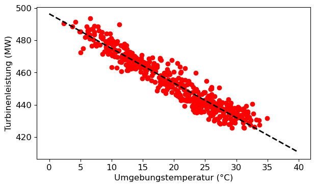
df_pp.corr()| Ambient_Temperature | Vacuum | Ambient_Pressure | Relative_Humidity | Power_Output | |
|---|---|---|---|---|---|
| Ambient_Temperature | 1.000000 | 0.844107 | -0.507549 | -0.542535 | -0.948128 |
| Vacuum | 0.844107 | 1.000000 | -0.413502 | -0.312187 | -0.869780 |
| Ambient_Pressure | -0.507549 | -0.413502 | 1.000000 | 0.099574 | 0.518429 |
| Relative_Humidity | -0.542535 | -0.312187 | 0.099574 | 1.000000 | 0.389794 |
| Power_Output | -0.948128 | -0.869780 | 0.518429 | 0.389794 | 1.000000 |
Regression
X = df_pp.drop(columns='Power_Output').values  # Features
y = df_pp.Power_Output.values  # Target

n_splits = 50
n_neighbors = 8
mean_test_scores = []
mean_train_scores = []

from sklearn.model_selection import train_test_split
from sklearn.neighbors import KNeighborsRegressor

for j in range(n_neighbors):
    test_scores = []
    train_scores = []
    for i in range(n_splits):
        X_train, X_test, y_train, y_test = train_test_split(X, y, random_state=i)
        knn = KNeighborsRegressor(n_neighbors=j + 1)  # Definition des Algorithmus
        knn.fit(X_train, y_train)  # Trainieren des Algorithmus
        train_scores.append(knn.score(X_train, y_train))
        test_scores.append(knn.score(X_test, y_test))
    mean_test_scores.append(np.mean(test_scores))
    mean_train_scores.append(np.mean(train_scores))

# print(mean_test_scores)
# print(mean_train_scores)
print('Die optimale Anzahl an Nachbarn ist=', np.argmax(mean_test_scores) + 1)
Die optimale Anzahl an Nachbarn ist= 6neighbors_arr = np.arange(1, n_neighbors + 1, 1)
# print(neighbors_arr)
plt.figure()
plt.plot(neighbors_arr, mean_test_scores,
color='red', marker='o', label='Test Scores')
plt.plot(neighbors_arr, mean_train_scores,
color='black', marker='o', label='Train Scores')
plt.ylim(0, 1.1)
plt.xticks(np.arange(1, n_neighbors + 1, 1))
plt.xlabel('Anzahl an Nachbarn')
plt.ylabel('Mittlere Scores')
plt.legend(loc=4)
plt.grid(True)
plt.tight_layout()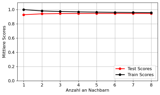
print(mean_test_scores[5])
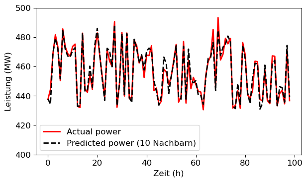
y_n10 = knn.predict(X_test)
knn = KNeighborsRegressor(n_neighbors=1) # Definition des Algorithmus
knn.fit(X_train, y_train) # Trainieren des Algorithmus
y_n1 = knn.predict(X_test)0.9458078675538566plt.figure()
plt.plot(y_test[-100:-1], color='red', label='Actual power')
plt.plot(y_n10[-100:-1], color='black', ls='dashed',
label='Predicted power (10 Nachbarn)')
# plt.plot(y_n1[-10:-1], color='blue', ls='dashdot',
# label='Predicted power (1 Nachbar)')
plt.ylim(400, 500)
plt.xlabel('Zeit (h)')
plt.ylabel('Leistung (MW)')
plt.legend()
plt.tight_layout()