
Vorlesung
Contents
Vorlesung#
Warum Python für wissenschaftliches Rechnen?#
Python ist eine freie, offene, plattformunabhängige, üblicherweise interpretierte, höhere Programmiersprache. Python Code ist gut lesbar und einfach zu lernen. Es gibt sehr viele Pakete und Einsatzgebiete für Python, siehe PyPI - the Python Package Index. Für den Bereich des wissenschaftlichen Rechnens sind insbesondere die SciPy-Pakete nützlich. Python erfreut sich einer großen und wachsenden Beliebtheit und besitzt daher eine umfangreiche und breitgefächert Community. So ziemlich jedes Problem mit Lösung/en findet man z. B. unter stackoverflow. Der Name bezieht sich übrigens auf die englische Komikergruppe Monty Python.
Nachfolgende Lehrveranstaltungen, die ebenfalls Python verwenden:
IDI:
im 4. Semester: Lineare Algebra und Operations Research
im 5. Semester: Angewandte Statistik und Data Analytics
UMW:
im 1. Semester: Mathematik für Umwelttechnik
im 2. Semester: Lineare Algebra und Operations Research
im 3. Semester: Angewandte Statistik
Zu den Alternativen im Bereich wissenschaftliches Rechnen zählen
Julia: frei, offen und plattformunabhängig
R: frei, offen und plattformunabhängig
Matlab: kommerziell
Mathematica: kommerziell
Es gibt, grob gesagt, zwei Typen von Entwicklungsumgebungen:
Ein Text-Editor kombiniert mit der Kommandozeile (englisch: command prompt, console, terminal). Entwicklungsumgebungen wie Thonny, Spyder, Visual Studio Code oder PyCharm kombinieren beides und mehr in einer Applikation.
Wir verwenden die web-basierte, interaktive, literate programming Entwicklungsumgebung JupyterLab, die neben Python noch viele andere Programmiersprachen mittels Jupyter-Notebooks untersützt. Im Wikipedia-Eintrag zum Projekt Jupyter steht (Stand 2020-06-18) unter anderem: “Das Jupyter Notebook hat sich als Benutzeroberfläche für Cloud Computing verbreitet. Große Cloud-Anbieter haben angepasste Tools für Cloud-Anwender entwickelt. Beispiele dafür sind Amazon SageMaker, Googles Colaboratory und Microsofts Azure Notebook.”
Installation#
Python und Python Pakete können auf sehr unterschiedliche Art und Weise installiert werden. Wir verwenden die von vielen empfohlene Variante der Python Distribution Anaconda. Um die Anaconda Distribution zu installieren, folgen Sie den Hinweisen entsprechend Ihrem Betriebssystem.
JupyterLab#
Starten Sie anschließen JupyterLab via dem Anaconda Navigator oder einfacher über eine Kommandozeile mit dem Befehl jupyter lab. Das meiste der Oberfläche ist selbsterklärend.
Wenn Sie ein (neues) Jupyter-Notebook (Dateiendung .ipynb) starten, wird ein Kernel gestartet. Der Kernel führt Ihre Python Befehle aus und beeinhaltet alle verwendeten Objekte (Variablen, Funktionen, Pakete etc.).
Achtung: Verwenden Sie generell für Ordner- und und Dateinamen keine Umlaute, keine Sonderzeichen und keine Leerzeichen!
Ein Jupyter-Notebook besteht aus einer Liste von Zellen (engl. cells).
Zellen können im Command Mode oder im Edit Mode bearbeitet werden.
Die wichtigsten zwei Zelltypen sind Code und Markdown.
Code Zellen:
Wir schreiben unseren Python Code in die Code-Zellen eines Jupyter-Notebooks. Zum Ausführen des Codes einer Code-Zelle drücken Sie
Strg+ReturnoderShift+Return. Bei der ersten Variante bleibt der Fokus auf der Code-Zelle, bei der zweiten springt man in die nächste Zelle.Der Rückgabewert des letzten Befehls einer Code Input-Zelle wird in einer folgenden Code Output-Zelle ausgegeben. Sie können die Ausgabe mit einem Strichpunkt am Ende des letzten Befehls unterdrücken.
Kommentare beginnen mit dem Rautezeichen
#.Funktionen haben runde Klammern. Hilfe z. B. zur Funktion
printerhalten Sie durchhelp(print)oderprint?oder SHIFT-TAB drücken, wenn der Cursor nach der ersten runden Klammer vonprint()steht.Eine Liste der von Ihnen definierten Variablen erhalten Sie mit dem magic command
%whos. Löschen einzelner Variablen, hier z. B. der Variablex, erfolgt mit dem Befehldel(x). Löschen aller selber definierten Variablen erfolgt mit dem Befehl%reset -s.Tipp: Verwenden Sie die Tabulator-Vervollständigung beim Coden!
Tipp: Mit der Tastenkombination
Strg+Iöffnet sich der sehr hilfreiche Contextual Help Tab.Tipp: Öffnen Sie eine Console für Ihr Notebook, um außerhalb des Notebooks interaktiv Befehle im Namespace des Notebook-Kernels auszuführen.
Markdown Zellen: Markdown ist eine vereinfachte Auszeichnungssprache, die bereits in der Ausgangsform ohne weitere Konvertierung leicht lesbar ist. Sie können in Markdown sehr leicht folgenden strukturierten Text erstellen:
Überschriften: Rautesymbol(e) vor der Überschrift
Listen: mit Minus-, Plus- oder Sternzeichen
Links: mit Syntax
[Name](URL)Bilder: mit Syntax
Mathematische Formeln wie z. B. \(K = \frac{mv^2}{2}\) via dem LaTeX-Code
$K = \frac{mv^2}{2}$Tipp: Cheatsheet
Keyboard Shortcuts
Die Keyboard Shortcuts sind in den Menüs neben den Auswahlen angegeben. Hier eine persönliche Auswahl:
Shortcut |
Effekt |
|---|---|
Ctrl+s |
save notebook |
Ctrl+Shift+q |
close and shutdown notebook |
Ctrl+f |
Find |
Enter |
enter edit mode |
Escape |
enter command mode |
Ctrl+Enter |
run cell |
Shift+Enter |
run cell and got to cell below |
Alt+Enter |
run cell and insert a new cell below |
Ctrl+b |
toggle left sidebar |
in edit mode: Ctrl+Shift+- |
split cell |
in command mode: m |
set cell type to markdown |
in command mode: y |
set cell type to code |
in command mode: d d |
delete cell |
in command mode: z |
undo deleting of cell |
in command mode: a |
insert cell above |
in command mode: b |
insert cell below |
in command mode:Shift+m |
merge selected cells |
in command mode: x/c/v |
cut/copy/paste cells |
in command mode: UP/DOWN arrow |
selected previous/next cell |
in command mode: i+i |
interrupt kernel |
in command mode: 0+0 |
restart kernel |
in command mode: Shift+l |
toggle all line numbers |
Bevor Sie JupyterLab beenden, vergessen Sie nicht, Ihre Jupyter-Notebooks zu speichern, zu schließen sowie die zugehörigen Kernel herunterzufahren. Wenn Sie JupyterLab von der Kommandozeile gestartet haben, beenden Sie JupyterLab mit zweimal Strg+C in der selben Kommandozeile.
Exportieren: Sie könne Jupyter-Notebooks über den Menüeintrag File/Export Notebook As oder über Systembefehle in andere Dateiformate exportieren. Systembefehle können Sie in einem System-Terminal, im Anaconda Command Prompt ausführen, oder in einer Codezelle, wenn Sie ein Rufezeichen vor den Systembefehl setzen. Hier eine Auswahl:
HTML: Systembefehl
jupyter nbconvert Mein_Notebook.ipynbPDF: Systembefehl
jupyter nbconvert --to pdf Mein_Notebook.ipynbLaTeX: Systembefehl
jupyter nbconvert --to latex Mein_Notebook.ipynbPython-Script: Systembefehl
jupyter nbconvert --to script Mein_Notebook.ipynb
Unter nbconvert finden Sie die Syntax für noch weitere Outputformate und Infos zu evtl. Zusatzsoftware, die für die Konvertierung notwendig ist.
Navigationsbefehle im Dateisystem: Für die Arbeit in einem System-Terminal, dem Anaconda Command Prompt oder in einer Codezelle sind oft folgende Navigationsbefehle nützlich:
pwd: print working/current directorylsoderdir: list files in current directorycd DIR: change into absolute or relative directory DIRcd ..: change to parent directory
Extensions: Folgende der vielen JupyterLab Extensions könnten Sie interessieren:
Noch ein Tipp zum Schluss: Schauen Sie mal in diese Liste von Jupyter Notebooks rein.
Einführung in Python für wissenschaftliches Rechnen#
Die folgende Einführung lehnt sich stark an die Kapitel 1 bis 4 des empfehlenswerten Buchs “Programming for Computations - Python. A Gentle Introduction to Numerical Simulations with Python 3.6.” von Svein Linge und Hans Petter Langtangen, 2. Auflage, 2020, an. Hier der Link zum Verlag.
Weitere nützliche Quellen:
Erste Schritte#
Wir schreiben unseren Python Code in die Code-Zellen eines Jupyter-Notebooks. Zum Ausführen des Codes einer Code-Zelle drücken Sie Strg+Return oder Shift+Return. Bei der ersten Variante bleibt der Fokus auf der Code-Zelle, bei der zweiten springt man in die nächste Zelle.
Hinweis: Um Ihren Code bei Bedarf außerhalb der JupyterLab-Umgebung auszuführen, können Sie
Ihr Jupyter-Notebook
mynotebook.ipynbin ein Python Script mit Endung.pyexportieren und anschließend von einem System-Terminal aus mitpython mynotebook.pystarten oderin einem System-Terminal
jupyter nbconvert --to notebook --execute mynotebook.ipynbverwenden.
Code-Kommentare beginnen mit dem Rautezeichen #. Funktionen haben immer runde Klammern. Das Potenzieren von Zahlen wird mit ** gemacht.
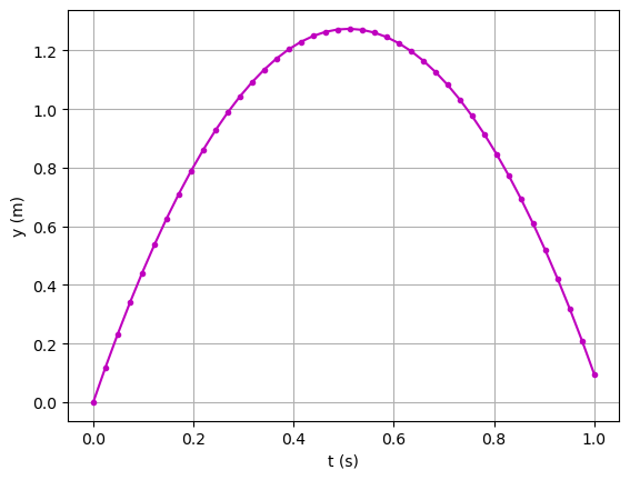
Hier ein erstes Beispiel: Der Code berechnet die Höhe \(y(t) = v_0 t - \frac{1}{2}gt^2\) eines Balls zum Zeitpunkt \(t \geq 0\), der zum Zeitpunkt \(t=0\) aus der Höhe \(y = 0\) mit der Geschwindigkeit \(v_0\) vertikal in die Höhe geworfen wird.
# program for computing the height of a ball in vertical motion

v0 = 5     # initial velocity in m/s
g  = 9.81  # acceleration of gravity in m/s^2
t  = 0.6   # time in s

y = v0*t - 0.5*g*t**2  # vertical position in m

print(f"At time t = {t} s the ball is at height y(t) = {y} m.")  # formated printing
At time t = 0.6 s the ball is at height y(t) = 1.2342 m.
Um Funktionen außerhalb der Python Standard Library, in der sich z. B. die Funktion print befindet, zu verwenden, importieren wir die gewünschten Python Pakete in den Namespace unseres Jupyter-Notebooks. Die Pakete NumPy und Matplotlib verwenden wir unter anderen in der Lehrveranstaltung.
# imports of packages into the namespace:
import numpy as np
import matplotlib.pyplot as plt
Die Funktionen und Module des Pakets numpy können nach dem obigen Import mit np.* angesprochen werden. Analoges gilt für die Funktionen von matplotlib.pyplot.
Mit NumPy können wir die Berechnung der vertikalen Position des Balls vektorisieren, und mit Matplotlib können wir diese grafisch darstellen.
t = np.linspace(0, 1, 42)

y = v0*t - 0.5*g*t**2

plt.plot(t, y, '.-m') # plots all y coordinates vs. all t coordinates
plt.xlabel("t (s)")   # places the text t (s) on x-axis
plt.ylabel("y (m)")   # places the text y (m) on y-axis
plt.grid(True)
Jetzt aber der Reihe nach!
Import von Paketen#
Anstatt das gesamte Paket some_package mit import some_package as some_prefix mit einem selbstgewählten Präfix some_prefix zu importieren, können auch einzelne Funktionen importiert werden.
from numpy import linspace, pi

# after the import linspace and pi are part of the namespace, e. g.:
linspace(0, 5, 11)
array([0. , 0.5, 1. , 1.5, 2. , 2.5, 3. , 3.5, 4. , 4.5, 5. ])
from numpy import cos as cosinus

cosinus(pi)
-1.0
Für den Import von Paketen müssen nicht unbedingt Präfixe wie z. B. np vergeben werden.
import numpy

numpy.linspace(0, 5, 11)
array([0. , 0.5, 1. , 1.5, 2. , 2.5, 3. , 3.5, 4. , 4.5, 5. ])
Achtung: Es ist nicht empfohlen, alle Funktionen und Module eines Pakets mit einem Import vom Typ from math import * in den Namespace zu importieren! Warum?
Datentypen - eine Auswahl#
Von den integrierten Datentypen verwenden wir die unten angeführten. Dabei besprechen wir deren Funktionalitäten nicht vollständig!
String: immutable
x = "Hello World"  # or 'Hello World'
print(type(x))
print("Applied " + "Mathematics") # adding is concatenating
<class 'str'>
Applied Mathematics
Integer: immutable
x = 42
print(type(x))
<class 'int'>
Float: immutable
# float is short for floating point number

x = 42.123456789
print(type(x))
<class 'float'>
print(type(12/3)) # result is of type float
<class 'float'>
print(4/4*3)
print(4/(4*3))  # do not forget the brackets if you wanted this.
3.0
0.3333333333333333
# computations:

print(4.5 + 1.5)  # addition
print(4.5 - 5)    # subtraction
print(2*7.1)      # multiplication
print(2**5)       # exponentiation
print(7.5/3)      # division
print(7.5//3)     # floor division, integer division
print(7.5%3)      # remainder, modulo
6.0
-0.5
14.2
32
2.5
2.0
1.5
List: mutable
# A list is a collection which is ordered and changeable (= mutable).

x = ['Eric', 42, 0.3]
print(type(x))
print(len(x))  # length, i. e. number of items, of the list
<class 'list'>
3
# accssing list items:
print(x[0])     # Python starts counting with 0!
print(x[1:3])   # item with index 1 included, item with index 3 excluded!
print(x[:2])    # items up to index 2 excluded
print(x[1:])    # items starting from index 1 included
print(x[-1])    # last item
print(x[-2])    # second last item
print(x[-2:])   # from the end up to second last item included
print(x[-2:-1]) #  should be clear now
Eric
[42, 0.3]
['Eric', 42]
[42, 0.3]
0.3
42
[42, 0.3]
[42]
# With the dot notation methods of the object can be accessed.
x.append(137)
x
['Eric', 42, 0.3, 137]
# lists can also be added and multiplied:
x = ['Eric', 42, 0.3]
print(x + ['John', 137])
print(2*x)
['Eric', 42, 0.3, 'John', 137]
['Eric', 42, 0.3, 'Eric', 42, 0.3]
Tuple: immutable
# A tuple is a collection which is ordered and unchangeable (= immutable).

x = ('Eric', 42, 1/3)
print(type(x))
print(x[1])
# But x has for example no append method.
# you can make it a list with
list(x)
<class 'tuple'>
42
['Eric', 42, 0.3333333333333333]
Dictionary: mutable
x = {"name" : "Eric",
     "age"  : 42}
print(type(x))
<class 'dict'>
# accessing dictionary items:
x['name']
'Eric'
# adding dict items:

x['course'] = 'AM'
x
{'name': 'Eric', 'age': 42, 'course': 'AM'}
Boolean: immutable
# boolean:

print(type(True))
print(type(False))
print(4 == 12/3)
print(4 >= 3)
print(4  < 3)
print(4 != 3)
print(42 in ['Eric', 42, 1/3])
<class 'bool'>
<class 'bool'>
True
True
False
True
True
Achtung! Zu den unveränderlichen (immutable) Objekten zählen integers, floats, strings und andere, während Numpy Arrays (siehe unten) und Listen Beispiele für veränderliche (mutable) Objekte sind. Das hat folgende wichtige Auswirkungen:
x = 1   # integer is immutable
y = x
y = 4
print(x)
1
# however:
x = [1, 2, 3]   # list is mutable
y = x   # Python creates a reference to the mutable object x
y[0] = 4
print(x)
[4, 2, 3]
# workaround with copying values:
x = [1, 2, 3]
y = x.copy()   # Python creates a new object y
y[0] = 4
print(x)
[1, 2, 3]
NumPy Arrays, short arrays: mutable
1-dimensionale Arrays für Vektorrechnung
2-dimensionale Arrays für Matrizenrechnung
x = np.array([1, 2.1, -5])
print(x)
print(type(x))
print(len(x))     # length, i. e. number of items
print(np.ndim(x)) # number of dimensions
[ 1.   2.1 -5. ]
<class 'numpy.ndarray'>
3
1
# accssing list items works the same as with lists:
print(x[0])     # Python starts counting with 0!
print(x[1:3])   # item with index 1 included, item with index 3 excluded!
print(x[:2])    # items up to index 2 excluded
print(x[1:])    # items starting from index 1 included
print(x[-1])    # last item
print(x[-2])    # second last item
print(x[-2:])   # from the end up to second last item included
print(x[-2:-1]) # should be clear now
1.0
[ 2.1 -5. ]
[1.  2.1]
[ 2.1 -5. ]
-5.0
2.1
[ 2.1 -5. ]
[2.1]
# With the dot notation many methods be accessed.
# Use the TAB-key after the dot to see them! Here' an example:
x.mean()
-0.6333333333333333
# Arrays can also be added and multiplied,
# but now in the sense of vector algebra!
y = np.array([3, -1.9, 42])

x + y # vector addition: elementwise!
array([ 4. , 0.2, 37. ])
print(x)
print(x + 100)   # adding a scalar to all elements
[ 1.   2.1 -5. ]
[101.  102.1  95. ]
3*x # multiplying a scalar to all elements
array([ 3. , 6.3, -15. ])
Das innere Produkt zweier Vektoren wird im Englischen oft “dot product” genannt.
np.dot(x, y)
-210.99
# alternatively with the @ operator:
x@y
-210.99
np.cross(x, y) # cross product: only für vectors with 3 elements
array([ 78.7, -57. , -8.2])
x*x # caution: elementwise!
array([ 1. , 4.41, 25. ])
x/x # elementwise!
array([1., 1., 1.])
x**3 # elementwise!
array([ 1. , 9.261, -125. ])
# constructors:

x = np.arange(start = 0, stop = 5, step=2)
print(x)

x = np.linspace(start = 0, stop = 5, num=11)
print(x)

x = np.zeros(4)
print(x)

x = np.ones(7)
print(x)
[0 2 4]
[0.  0.5 1.  1.5 2.  2.5 3.  3.5 4.  4.5 5. ]
[0. 0. 0. 0.]
[1. 1. 1. 1. 1. 1. 1.]
# The thing about copying ... :

x = np.array([1,2,3])
y = x
y[0] = 4
print(x)

x = np.array([1,2,3])
y = x.copy()
y[0] = 4
print(x)
[4 2 3]
[1 2 3]
# 2-dim arrays, aka matrices:

M = np.array([[1, 2, 3],
              [4, 5, 6]])

print(M)
print(np.ndim(M)) # number of dimensions, number of square brackets
print(M.shape)    # number of rows and number of columns
[[1 2 3]
 [4 5 6]]
2
(2, 3)
# accessing items and slices:
print(M[1,2])    # select one element
print(M[1,:])    # select row as 1-dim array
print(M[:,0])    # select columns as 1-dim array
print(M[:,[0]])  # select columns as 2-dim array
6
[4 5 6]
[1 4]
[[1]
 [4]]
Overview of mutable and immutable data types:
mutable data types: list, dictionary, array, …
immutable data types: int, float, bool, string, tuple, …
Formatiertes Drucken#
Wir verwenden “f-strings” für das formatierte Drucken. Zwei weitere Methoden werden z. B. im Buch von Linge und Langtangen beschrieben. f-strings beginnen mit einem f vor den Anführungszeichen, die den string kennzeichnen. Variablenwerte werden in geschwungenen Klammern eingebunden. Zeichenketten (=strings), die über mehrere Zeilen laufen, können mit dreifachen Anführungszeichen geschrieben werden. \n bewirkt eine neue Zeile im Ausdruck. Mehr zu f-strings finden Sie z. B. im Python f-string tutorial.
my_name  = "Klaus"
my_age   = 47
my_float = 123.123456789

print(f"Hallo! My name is {my_name}.")
print(f"Two of my objects:\n  {my_name = }\n  {my_age = }.") # self-documenting expression
print(f"I am {my_age} years old. These are about {my_age*365} days.")
print(f"""My number in different formats:
  {my_float:.3f} or
  {my_float:10.5f} or
  {my_float:.3e} or
  {my_float:10.2e}""")
Hallo! My name is Klaus.
Two of my objects:
  my_name = 'Klaus'
  my_age = 47.
I am 47 years old. These are about 17155 days.
My number in different formats:
  123.123 or
   123.12346 or
  1.231e+02 or
    1.23e+02
Grafiken#
Wir werden nur wenige Beispiele in diesem Abschnitt aufzeigen. Die große Vielfalt an grafischen Darstellungsmöglichkeiten mit dem Python-Paket Matplotlib finden Sie z. B. unter Matplotlib Gallery. Es gibt neben Matplotlib noch viele andere Grafik-Pakete. Interaktive Grafiken können Sie z. B. mit ipywidgets erstellen.
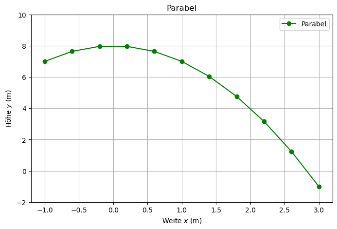
x = np.linspace(-1, 3, num = 11)
y = -x**2 + 8

plt.figure(figsize=(8,5))
plt.plot(x, y, 'o-g', label='Parabel')
plt.xlabel('Weite $x$ (m)')
plt.ylabel('Höhe $y$ (m)')
plt.ylim(-2, 10)
plt.title('Parabel')
plt.legend(numpoints=1, loc='best')
plt.grid(True)

plt.savefig('/home/kr/lehre/am/web/1_Python/Parabel.pdf')
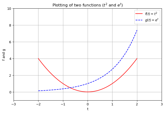
t = np.linspace(-2, 2, 100)
f_values = t**2
g_values = np.exp(t)

plt.figure(figsize=(8,5))
plt.plot(t, f_values, 'r',
         t, g_values, 'b--')
plt.xlabel('t')
plt.ylabel('f and g')
plt.legend(['$f(t) = t^2$',
            '$g(t) = e^t$'])
plt.title('Plotting of two functions ($t^2$ and $e^t$)')
plt.grid(True)
plt.axis([-3, 3, -1, 10]);
Kontrollstrukturen#
for-Schleife: hat die Struktur
for loop_variable in iterable_object:
    <code line 1>
    <code line 2>
    etc.
# first code line after the loop
# example 1: iteration over a list

for item in ["1", 2, np.pi]:
    print(item)
1
2
3.141592653589793
# example 2: iteration over an array

v = np.linspace(0, 3, 7)
for x in v:
    print(x, end=", ")
0.0, 0.5, 1.0, 1.5, 2.0, 2.5, 3.0,
# example 3: using enumerate to get the indices too

my_list= ['Sokrates', 'Platon', 'Aristoteles']
for index, value in enumerate(my_list):
    print(f"{index + 1}. {value}")
1. Sokrates
2. Platon
3. Aristoteles
# list comprehension:

my_list_1 = [-x for x in np.arange(-3, 4)]
print(my_list_1)

my_list_2 = [-x for x in np.arange(-3, 4) if x < 0]
print(my_list_2)

my_list_3 = [-x if x < 0 else x for x in np.arange(-3, 4)]
print(my_list_3)
[3, 2, 1, 0, -1, -2, -3]
[3, 2, 1]
[3, 2, 1, 0, 1, 2, 3]
while-Schleife: hat die Struktur
while some_condition:
    <code line 1>
    <code line 2>
    etc.
# first code line after the loop
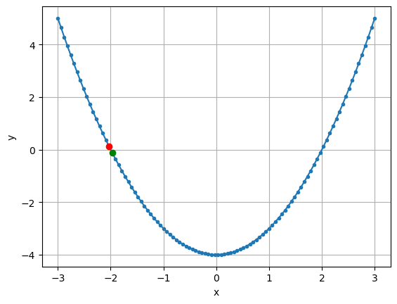
# find the first (i. e. in ascending order) data points nearest to zero:
x = np.linspace(-3, 3, num=100)
y = x**2 - 4

plt.plot(x, y, '.-')
plt.xlabel('x')
plt.ylabel('y')

ind = 0  # staring index, proceed to increasing values
sign_change = False
while not sign_change:
    old_sign = np.sign(y[ind])
    ind += 1
    new_sign = np.sign(y[ind])
    if new_sign != old_sign:
        sign_change = True

print(f"y[{ind -1}] = {y[ind - 1]}")
print(f"y[{ind   }] = {y[ind    ]}")
plt.plot(x[ind - 1], y[ind - 1], 'or')
plt.plot(x[ind    ], y[ind    ], 'og')
plt.grid(True)
y[16] = 0.12213039485766775
y[17] = -0.12029384756657491
if-elif-else-Abfragen: hat die Struktur
if condition_1:
    <code line 1>
    <code line 2>
    ...
elif condition_2: # optinonal
    <code line 1>
    <code line 2>
    ...
elif condition_3: # optinonal
    <code line 1>
    <code line 2>
    ...
else:             # optinonal
    <code line 1>
    <code line 2>
    ...
# First line after if-elif-else construction
T = 5 # select a water temperature in degree centigrade

if T <= 20:
    print("Do not swim. Too cold!")
elif T <= 36:
    print("Great, jump in!")
else:
    print("Do not swim. Too hot!")
Do not swim. Too cold!
Tipps:
Mit der
break-Anweisung gelangen Sie direkt zur ersten Codezeile nach einer Schleife.Mit der
continue-Anweisung fahren Sie direkt mit der nächsten Iteration fort.
Funktionen#
Eine Funktion hat die Struktur
def function_name(pos1, pos2, ..., kw1=default_1, kw2=default_2, ...):   # function header
    """This is a docstring"""         # function body
    <code line>                       # function body
    <code line>                       # function body
    ...                               # function body
    return result_1, result_2, ...    # last line in function body
# First line after function definition
Die return Zeile, die die Rückgabewerte definiert, und die Argumente pos1, ..., kw1 = ... sind jeweils optional. Eine Funktion kann daher auch so aussehen:
def my_function():
    """function without arguments
    and without return values"""
    print("Ahoi!")
my_function()
Ahoi!
Der Doc-String ist der Hilfetext zur Funktion und kann aufgrund der dreifachen doppelten Anführungszeichen über mehrere Zeilen laufen.
help(my_function)
Help on function my_function in module __main__:

my_function()
    function without arguments
    and without return values
Argumente:
Die Argumente
pos1, pos2, ...sind sogenannte positional parameters.Die Argumente
kw1, kw2, ...sind sogenannte keyword parameters.
Positional parameters müssen vor keyword parameters angeführt werden.
Die Werte der Parameter, die beim Aufruf der Funktion übergeben werden heißen positional bzw. keyword arguments.
Die Werte default_1 und default_2 sind Default-Werte, die verwendet werden, wenn keine entsprechenden keyword arguments beim Aufruf der Funktion angegeben werden.
Hier ein Beispiel:
def my_greet(first_name, second_name, msg="Good morning!"):
    print(f"Hello {first_name} {second_name}! {msg}")
my_greet('Albert', 'Einstein')
my_greet('Albert', 'Einstein', msg='Good night!')
my_greet('Albert', 'Einstein', 'Good night!')
my_greet('Good night!', 'Albert', 'Einstein')  # gives no error, but is not what you intended!
my_greet(first_name="Albert", second_name='Einstein', msg="How do you do?")
my_greet("Albert", second_name='Einstein', msg="How do you do?")
my_greet(msg = "How do you do?", first_name="Albert", second_name='Einstein')
my_greet(second_name='Einstein', first_name="Albert", msg = "How do you do?")
# my_greet(msg="How do you do?", "Albert", "Einstein") # gives "SyntaxError: positional argument follows keyword argument"!
Hello Albert Einstein! Good morning!
Hello Albert Einstein! Good night!
Hello Albert Einstein! Good night!
Hello Good night! Albert! Einstein
Hello Albert Einstein! How do you do?
Hello Albert Einstein! How do you do?
Hello Albert Einstein! How do you do?
Hello Albert Einstein! How do you do?
Erkenntnisse:
Keyword arguments können auch ohne keyword angegeben werden.
Es ist möglich, die Namen von positional parameters als keywords zu verwenden.
Die Reihenfolge von keyword arguments kann geändert werden.
Eine Funktion kann mit positional oder mit keyword arguments oder aus einer Mischung aufgerufen werden. Bei der Mischvariante müssen die positional arguments jedoch zuerst angeführt werden müssen.
Solange in einem Funktionsaufruf für alle Argumente keywords verwendet werden, kann eine beliebige Reihenfolge der Argumente verwendet werden.
Geltungsbereich von Variablen (engl. Scope of Variables):
if "y" in locals():
    del(y)
k =   2  # global variable defined in the main program
d = 100  # global variable defined in the main program

def my_line_value(x):
    # The global variables k and d are known from "outside".
    k = 10  # k is now also the name of a local variable.
    # The assignment k = 10 changes only the local variable inside the function.
    # The "name-brother" global variable outside is not affected!
    print(f"inside values: k = {k}, d = {d}")
    y = k*x + d
    print(f"inside computation {y} = {k}*{x} + {d}")
    return y

x = 3

print(f"outside values before function call: k = {k}, d = {d}")
print(f"return value of input {x}: {my_line_value(x)}.")
print(f"outside values after function call: k = {k}, d = {d}")
# print(y) # gives "NameError: name 'y' is not defined"
outside values before function call: k = 2, d = 100
inside values: k = 10, d = 100
inside computation 130 = 10*3 + 100
return value of input 3: 130.
outside values after function call: k = 2, d = 100
Achtung: Veränderliche (d. h. mutable) äußere Objekte werden in Funktionen geändert!
x = [1, 2]  # mutable object
print(f"outside value: {x = }")

def change(y):
    y[0] = 4
    print(f"inside value:  {y = }")

change(x)
print(f"outside value: {x = }")
outside value: x = [1, 2]
inside value:  y = [4, 2]
outside value: x = [4, 2]
# Auch ohne Übergabe:

x = [1, 2]  # mutable object
print(f"outside value: {x = }")

def change():
    x[0] = 4
    print(f"inside value:  {x = }")

change()
print(f"outside value: {x = }")
outside value: x = [1, 2]
inside value:  x = [4, 2]
outside value: x = [4, 2]
# Aber:

x = 1  # immutable object
print(f"outside value: {x = }")

def change():
    x = 4
    print(f"inside value:  {x = }")

change()
print(f"outside value: {x = }")
outside value: x = 1
inside value:  x = 4
outside value: x = 1
Lambda Funktionen: sind eine Möglichkeit, auf kompakte Art “Einzeiler”-Funktionen zu definieren.
g = lambda x: x**2
# is equivalent to:
# def g(x):
#     return x**2

g(3)
9
Allgemeine Form einer Lambda Funktion:
function_name = lambda arg1, arg2, ... : <some_expression>
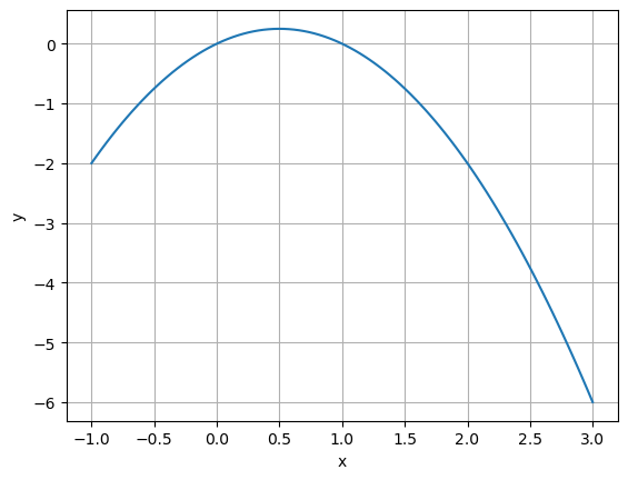
Funktionen als Argumente von Funktionen:
def my_plot(fct, start=-1, stop=3, legend=True):
    x = np.linspace(start, stop, num=100)
    y = fct(x)
    plt.plot(x, y, label=fct.__name__)
    plt.xlabel('x')
    plt.ylabel('y')
    if legend:
        plt.legend()
    plt.grid(True)
my_plot(np.sin, 0, 2*np.pi)
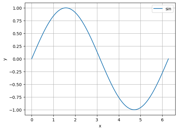
my_plot(lambda x: x - x**2, legend=False)
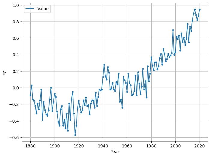
Daten IO#
Es gibt sehr viele Arten von Daten und Dateitypen. Wir beschränken uns hier auf das Laden und Speichern von einfachen CSV-Dateien. Als Beispiel nehmen wir die global temperature anomalies with respect to the 20th century average, genauer die dort bereitgestellte csv-Datei data.csv. Anstatt die Daten Zeile für Zeile einzulesen und zu parsen, verwenden wir das sehr mächtige und allen Data Scientists empfehlenswerte Paket pandas.
import pandas as pd
filepath = "/home/kr/lehre/am/web/1_Python/data.csv"
df = pd.read_csv(filepath, skiprows=4, index_col=0) # read file into a pandas DataFrame
df
| Value | |
|---|---|
| Year | |
| 1880 | -0.09 |
| 1881 | 0.03 |
| 1882 | -0.14 |
| 1883 | -0.16 |
| 1884 | -0.22 |
| ... | ... |
| 2016 | 0.95 |
| 2017 | 0.88 |
| 2018 | 0.82 |
| 2019 | 0.87 |
| 2020 | 0.95 |
141 rows × 1 columns
# We can directly plot the DataFrame ...

df.plot(figsize=(8,6), grid=True, marker='.')
plt.ylabel('°C');
# ... or we convert the data to data types we already know ...

years  = df.index.values     # to numpy array
values = df['Value'].values  # to numpy array

# ... and plot these:

plt.figure(figsize=(8,6))
plt.plot(years, values, '.-', label='Values')
plt.xlabel('Year')
plt.ylabel('°C')
plt.legend()
plt.grid(True)

# exporting data to files:

# from DataFrame to Excel:
my_filepath = "/home/kr/lehre/am/web/1_Python/data_exported_with_pandas.xlsx"
df.to_excel(my_filepath)

# from numpy array to csv:
my_filepath = "/home/kr/lehre/am/web/1_Python/data_exported_with_numpy.csv"
np.savetxt(my_filepath, values, delimiter=',') # using numpy