Code
import numpy as np
import matplotlib.pyplot as pltDie Aufgaben müssen in ILIAS als lauffähige und dokumentierte Jupyter Notebooks inkl. Datenfiles abgegeben werden. LP-Modellierungen können als eingescannte PDFs abgegeben werden.
Im Demand Side Management (DSM) werden unter anderem die Lasten von Verbrauchern direkt oder indirekt gesteuert, um z. B. ihre Gesamtlastspitze zu reduzieren oder ihre Gesamtlast einer nicht flexiblen (z. B. erneuerbaren) Erzeugung anzupassen.
Literaturhinweis: P. Palensky and D. Dietrich, “Demand Side Management: Demand Response, Intelligent Energy Systems, and Smart Loads,” IEEE Transactions on Industrial Informatics, vol. 7, no. 3, pp. 381–388, Aug. 2011, doi: 10.1109/TII.2011.2158841.
Wir betrachten fünf Verbraucher in Viertelstundenschritten über einen Tag. Der fixierte Verbrauch ist im Code unten angegeben. Die Flexibilität für die Verbraucher wird jeweils durch die gleiche, verlustfreie Batterie gegeben, deren Parameter unten angeführt sind. Die Gesamtlast der Verbraucher soll über den Tag möglichst der nicht flexiblen, angegeben PV-Erzeugung angepasst werden. Dabei wird die maximale absolute Abweichung zwischen Last und Erzeugung als Bewertung der Anpassung verwendet.
import numpy as np
import matplotlib.pyplot as pltdt = 0.25 # h
times = np.arange(start=0, stop=24 + dt, step=dt) # timestamps: 0, 0.25, 0.5, ..., 23.75, 24
periods = np.arange(start=0, stop=24, step=dt) # start times of periods: 0, 0.25, 0.5, ..., 23.75
# source: https://www.bdew.de/energie/standardlastprofile-strom/
demand = np.array([87.7, 81.5, 76.2, 71.0, 65.8, 60.5, 55.6, 51.5, 48.5, 46.4, 44.9, 43.7, 42.7,
41.8, 41.1, 40.6, 40.4, 40.4, 40.5, 40.6, 40.6, 40.6, 40.5, 40.6, 40.8, 41.6,
43.2, 46.1, 50.6, 56.7, 64.6, 74.2, 85.5, 97.9, 110.7, 123.4, 135.3, 145.9,
155.1, 162.4, 167.8, 171.8, 175.5, 179.6, 184.9, 190.5, 195.7, 199.1, 200.4,
198.8, 194.3, 186.7, 176.1, 163.9, 151.7, 141.3, 134.0, 129.1, 125.7, 122.7,
119.3, 115.5, 111.7, 107.8, 104.2, 101.1, 99.1, 98.4, 99.5, 102.1, 106.2,
111.7, 118.2, 125.5, 132.8, 139.8, 145.9, 150.7, 153.5, 153.9, 151.6, 147.4,
142.8, 139.1, 136.9, 135.8, 134.8, 132.8, 129.0, 123.7, 117.0, 109.3, 101.0,
92.3, 83.7, 75.7])
demand = demand/(np.sum(demand)*dt)*40 # demand load in kW, scaled to 40 kWh energy demand
# households:
num_of_households = 5 # number of households
# household load profiles:
np.random.seed(7)
demand_hh = np.zeros((num_of_households, len(periods)))
for h in range(num_of_households):
noise = np.random.normal(loc=0, scale=0.4, size=len(periods))
weights = np.exp(-.5*periods[:4])
demand_hh[h] = demand + np.convolve(noise, weights, mode='same')
# power generation:
pv_power = np.zeros_like(periods)
pv_power[6*4:6*4 + 12*4] = 25*np.sin(2*np.pi/(6*4) * periods[:12*4] ) # PV power in kW
plt.figure(figsize=(6, 5))
plt.subplot(2, 1, 1)
plt.step(periods, demand_hh.T, where='post', alpha=0.5)
plt.xlabel('time [h]')
plt.ylabel('power [kW]')
plt.legend([f'household {h}' for h in range(num_of_households)])
plt.grid()
plt.subplot(2, 1, 2)
plt.step(periods, demand_hh.sum(axis=0), where='post', label='total demand')
plt.step(periods, pv_power, where='post', label='PV power')
plt.xlabel('time [h]')
plt.ylabel('power [kW]')
plt.legend()
plt.grid()
plt.tight_layout()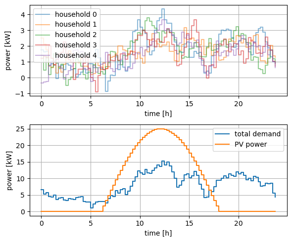
print(f"total demand energy = {demand_hh.sum()*dt:.2f} kWh")
print(f"total PV energy     = {pv_power.sum()*dt:.2f} kWh")
total demand energy = 189.37 kWh
total PV energy = 190.92 kWh# household battery parameters:
E_max = 20.0 # kWh, maximum energy level
E_start = 10.0 # kWh, starting energy level
E_end = 10.0 # kWh, final energy level
p_max = 10.0 # kW, maximum (dis-)charging power