Code
import numpy as np
import matplotlib.pyplot as plt
import pyomo.environ as pyoSie kommen mittags um 12 Uhr mit ihrem E-Mobil nach Hause und haben nun 8 Stunden Zeit, es wieder voll zu laden, da Sie abends um 20 Uhr eine längere Reise beginnen. Ihr E-Mobil hat eine Batterie mit einer Kapazität von 60 kWh, der aktuelle SoC (State of Charge) beträgt 40 %. Ihre Ladestation hat eine maximale Ladeleistung von 11 kW. Ihr Energieversorger bietet Ihnen einen zeitabhängigen Stromtarif mit den folgenden, stündlichen Energiepreisen in Cent/kWh für die kommenden acht Stunden an: 10, 8, 12, 13, 11, 10, 13, 14.
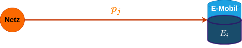
Fragen: Mit welchen, stündlich konstanten Ladeleistungen \(p_j\) sollen Sie Ihr E-Mobil laden, so dass Sie die Ladekosten minimieren? Wie hoch sind die minimalen Ladekosten? Wann ist Ihr E-Mobil voll geladen?
Vorgehen:
Zeitpunkte, Zeitperioden und ihre Indizierung:
Daten:
import numpy as np
import matplotlib.pyplot as plt
import pyomo.environ as pyodt = 1 # h
times = np.arange(start=12, stop=20 + 1, step=dt) # h, 12, 13, ..., 19, 20
time_indices = range(len(times))
period_indices = range(len(times) - 1)
prices = np.array([10, 8, 12, 13, 11, 10, 13, 14])
prices_ = np.array([10, 8, 12, 13, 11, 10, 13, 14, 14]) # append last price for step-plotting
plt.figure(figsize=(5, 3))
plt.step(times, prices_, where='post', color='red', marker='.')
plt.xlabel('time (h)')
plt.ylabel('price (Cent/kWh)')
plt.grid()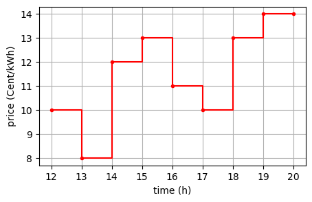
Entscheidungsvariablen:
Zielfunktion: Minimiere die Ladekosten in Cent: \[\min \sum_{j=0}^7 c_j p_j \Delta t\]
Nebenbedingungen:
model = pyo.ConcreteModel()

model.I = pyo.Set(initialize=time_indices)
model.J = pyo.Set(initialize=period_indices)

model.E = pyo.Var(model.I, bounds=(0.0, 60.0))
model.p = pyo.Var(model.J, bounds=(0.0, 11.0))

model.cost = pyo.Objective(expr=sum(prices[j]*model.p[j]*dt for j in model.J),
                          sense=pyo.minimize)

model.initial_energy = pyo.Constraint(expr = model.E[0] == 24.0)
model.final_energy = pyo.Constraint(expr = model.E[8] == 60.0)

@model.Constraint(model.I)
def charging(model, i):
    if i < 8:
        return model.E[i + 1] == model.E[i] + model.p[i]*dt
    else:
        return pyo.Constraint.Skip

# model.pprint()solver = pyo.SolverFactory('cbc')
# solver = pyo.SolverFactory('glpk')
# solver = pyo.SolverFactory('appsi_highs')
# solver = pyo.SolverFactory('gurobi')
results = solver.solve(model, tee=False)
print(f"status = {results.solver.status}")
print(f"minimal cost = {pyo.value(model.cost)/100.0:.2f} EUR")status = ok
minimal cost = 3.41 EURE_sol_dict = model.E.extract_values()
E_sol = [E_sol_dict[i] for i in time_indices]
p_sol_dict = model.p.extract_values()
p_sol = [p_sol_dict[j] for j in period_indices]
p_sol_ = np.concatenate( (p_sol, [p_sol[-1]]) )
plt.figure(figsize=(5, 8))
plt.subplot(3, 1, 1)
plt.step(times, prices_, where='post', marker='.', color='red')
plt.xlabel('Zeit [h]')
plt.ylabel('Preis [Cent/kWh]')
plt.grid(True)
plt.subplot(3, 1, 2)
plt.step(times, p_sol_, where='post', marker='.', color='blue')
plt.xlabel('Zeit [h]')
plt.ylabel('Leistung [kW]')
plt.grid(True)
plt.subplot(3, 1, 3)
plt.plot(times, E_sol, marker='.', color='green')
plt.xlabel('Zeit [h]')
plt.ylabel('Energie [kWh]')
plt.grid(True)
plt.tight_layout()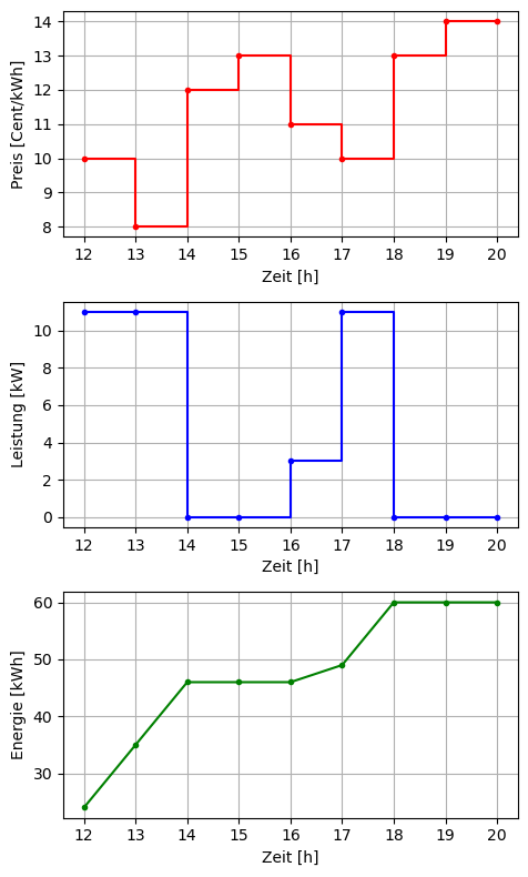
Das E-Mobil ist bereits um 18 Uhr vollgeladen.
price_mean = prices.mean()  # Cent/kWh
print(f"mean price = {price_mean:.2f} Cent/kWh")
mean price = 11.38 Cent/kWhcost_mean_price = price_mean*(60 - 24)/100 # EUR
cost_prices = pyo.value(model.cost)/100.0 # EUR
print(f"cost with varying prices = {cost_prices:.2f} EUR")
print(f"cost with constant price = {cost_mean_price:.2f} EUR")
print(f"absolute saving = {cost_mean_price - cost_prices:.2f} EUR")
print(f"relative saving = {(cost_mean_price - cost_prices)/cost_mean_price*100:.2f} %")cost with varying prices = 3.41 EUR
cost with constant price = 4.09 EUR
absolute saving = 0.68 EUR
relative saving = 16.73 %Das Ladeproblem kann auch mit dem “Valley/Water Filling” Algorithmus gelöst werden. Dabei werden zuerst die Stunden mit den niedrigsten Preisen in maximalem Umfang zum Laden verwendet.