Pyomo

Überblick

Wir verwenden in der Lehrveranstaltung das Python-Paket Pyomo. Pyomo ist ein Open-Source-Projekt und frei verfügbar. Pyomo ist eine algebraische Modellierungssprache zur benutzerfreundlichen Formulierung von mathematischen Optimierungsproblemen. Zum Lösen eines mit Pyomo formulierten Optimierungsproblems wird ein Solver benötigt. Pyomo unterstützt eine Vielzahl von kommerziellen und Open-Source-Solvern.

Links:

Pyomo Dokumentation zu Pyomo.
Hands-On Optimization with Python insbesodere Pyomo style guide.

Alternativen

In diesem Abschnitt geben wir einen Überblick über andere High-Level Software zur Formulierung von Optimierungsproblemen, weil:

Die Links führen Sie zu vielen, oft sehr guten Tutorials inkl. Code-Beispielen.
In Realprojekten ist es wichtig, das passende Software-Setting unter Berücksichtigung folgender Punkte auszuwählen: kommerziell versus open source, Schnittstellen zu Programmiersprachen, Benutzerfreundlichkeit, Performance etc.. Dafür sollte man seinen Überblick über die LP-Software aktuell halten.

Liste von bekannten Algebraischen Modellierungssprachen:

AMPL: you can find examples e. g. in the AMPL book
GAMS: for some simple examples see e. g.the GAMS Quick Start Tutorial
AIMMS: in AIMMS_modeling.pdf you find many examples and tricks
Mosel: for examples see e. g. the FICO Xpress Optimization Examples Repository
GNU MathProg where you can find a short example, see also GLPK and this online solver. The GNU MathProg language is a subset of the AMPL language.
OPL: for examples see e. g. the OPL Language User’s Manual
MPL: you can find examples e. g. here

Für Python gibt es unter anderem folgende Modellierungs- und Entwicklungsumgebungen für (MI)LPs:

SciPy LP and MILP with linprog and milp: open source solver and interface, modelling in matrix/vector form
CVXOPT: open source interface to own solver and other solvers, can also solve quadratic programs, user’s guide, see also cvxpy
gurobipy: interface to commercial Gurobi solver
Cplex: commercial solver and interface, academic license available
lp_solve: open source solver and interface
GLPK interfaces: open source solver and interfaces
Pyomo: open source interface to different solvers
PuLP: open source interface to own solver and other solvers documentation, github
linopy: open source interface to different solvers
Python-MIP: open source interface to different solvers
PySCIPOpt: interface to the SCIP Optimization Suite, scipbook
Optlang: open source interface to different solvers, github
PYMPROG: open source interface to different solvers

Solver

Liste der bekanntesten Solver:

CBC: open source solver
HiGHs: open source solver
GLPK: open source solver
SCIP Optimization Suite: non-commercial solver for mixed integer programming (MIP) and mixed integer nonlinear programming (MINLP)
lp_solve: open source solver
Gurobi: commercial solver, academic license available
Cplex: commercial solver and interface, academic license available
Xpress: commercial solver
Ipopt: open source software package fo large-scale nonlinear optimization, documentation

Installation

TIPP: Wir empfehlen die Installation von Pyomo und den Solvern in einer conda environment! Eine Anleitung dafür finden Sie hier in der Lehrveranstaltung Programmiertechniken.

Pyomo

using conda: conda install -c conda-forge pyomo
using pip: pip install pyomo

Solver

Windows

GLPK using conda: conda install -c conda-forge glpk
CBC: download the cbc zip-file for Windows from AMPL. Extract the zip-file and copy cbc.exe to the folder of your Python code. Use solver = pyo.SolverFactory('cbc.exe').
HiGHS: conda install -c conda-forge highs, and pip install highspy. Copy the file highs.exe from C:\Users\USERNAME\...\pkgs\highs-XY\Library\bin to the folder of your Python code.

macOS and Linux

GLPK: install GLPK with your package manager, or conda install -c conda-forge glpk
CBC: install CBC with your package manager, or conda install -c conda-forge coincbc.
HiGHS: install HiGHS with your package manager, or conda install -c conda-forge highs and pip install highspy.

Alle Plattformen

Gurobi: first install the gurobi solver using your students.fhv.at email account, cf. academic license. For the Python interface you have the following options:
- using conda: conda config --add channels https://conda.anaconda.org/gurobi, conda install gurobi
- using pip: pip install gurobipy

Tutorial

Beispiel: Butter und Eiscreme

Wir werden nun das folgende kleine LP mit Pyomo modellieren und mit verschiedenen Solvern lösen.

Fragestellung: Ein Bauer hat 3 Kühe, die in Summe 22 Gallonen (1 Gallone $\simeq$ 3.785 Liter) Milch pro Woche geben. Aus der Milch kann er Eiscreme und Butter machen. Er braucht 2 Gallonen Milch für 1 kg Butter und 3 Gallonen Milch für 1 Gallone Eiscreme. Es gibt keine Lagerrestriktionen für Butter. Er kann maximal 6 Gallonen Eiscreme lagern. Er hat 6 Arbeitsstunden pro Woche für die Herstellung zur Verfügung. Für 4 Gallonen Eiscreme benötigt er 1 Stunde, für 1 kg Butter benötigt er ebenfalls 1 Stunde. Die gesamte Produktion kann er zu folgenden Preisen verkaufen (vollständiger Absatz): 5 USD pro Gallone Eiscreme, 4 USD pro kg Butter. Seine Kosten belaufen sich auf 1.5 USD pro Gallone Eiscreme und 1 USD pro kg Butter. Wie viele Gallonen Eiscreme und wie viele kg Butter soll er herstellen, sodass er seinen Profit maximiert?

Modellierung:

Entscheidungsvariablen:

$x$: produzierte Gallonen Eiscreme
$y$: produzierte kg Butter

Zielfunktion: Maximiere den Profit $5x + 4y - (1.5 x + y) = 3.5x + 3y$.

Nebenbedingungen:

Lagerung von Eiscreme: $x \leq 6$
Arbeitszeit: $\frac{1}{4}x + y \leq 6$
verfügbare Milch: $3x + 2y \leq 22$
Positivität der Variablen: $x\geq 0, y\geq 0$

Das gesamte lineare Programm (LP):

\[ \begin{aligned} \text{max.}\; 3.5 x + 3 y & \\ \text{s. t.}\; x & \leq 6 \\ \frac{1}{4}x + y & \leq 6 \\ 3x + 2y & \leq 22 \\ x & \geq 0 \\ y & \geq 0 \end{aligned} \]

Quellen:

Problemstellung: Ferris, Mangasarian, Wright: Linear Programming with MATLAB. SIAM (Society for Industrial and Applied Mathematics), 2008
Pyomo: A basic Pyomo model.

Code

# The module pyomo.environ provides the components 
# most commonly used for building Pyomo models:
import pyomo.environ as pyo

Code

# create a model with an optional problem title:
model = pyo.ConcreteModel("butter_and_ice_cream")

Code

# Display the model. Currently the model is empty:
model.display()

Model butter_and_ice_cream

  Variables:
    None

  Objectives:
    None

  Constraints:
    None

Entscheidungsvariablen:

Standardmäßig ist die Domäne die Menge aller reellen Zahlen. Andere häufig verwendete Domänen sind pyo.NonNegativeReals, pyo.NonNegativeIntegers und pyo.Binary, siehe hier.
bounds ist ein optionales Schlüsselwort zur Angabe eines Tupels, das Werte für die untere und obere Schranke enthält.

Code

model.x = pyo.Var(bounds=(0, 6))
model.y = pyo.Var(domain=pyo.NonNegativeReals)

# display updated model:
model.display()

Model butter_and_ice_cream

  Variables:
    x : Size=1, Index=None
        Key  : Lower : Value : Upper : Fixed : Stale : Domain
        None :     0 :  None :     6 : False :  True :  Reals
    y : Size=1, Index=None
        Key  : Lower : Value : Upper : Fixed : Stale : Domain
        None :     0 :  None :  None : False :  True : NonNegativeReals

  Objectives:
    None

  Constraints:
    None

Ausdrücke (engl. expressions): Pyomo-Ausdrücke sind mathematische Formeln, die Entscheidungsvariablen enthalten. Pyomo-Ausdrücke werden verwendet, um die Zielfunktion und Nebenbedingungen zu definieren.

Code

# create some expressions:
model.revenue = 5*model.x + 4*model.y
model.cost = 1.5*model.x + 1*model.y

# expressions can be printed:
print(model.revenue)
print(model.cost)

5*x + 4*y
1.5*x + y

Zielfunktion:

Code

# set the objective function with another expression:
model.profit = pyo.Objective(expr = model.revenue - model.cost, sense = pyo.maximize)

# alternatively:
# model.profit = pyo.Objective(expr = 3.5*model.x + 3*model.y, sense = pyo.maximize)

Code

# pretty print the model:
model.pprint()

2 Var Declarations
    x : Size=1, Index=None
        Key  : Lower : Value : Upper : Fixed : Stale : Domain
        None :     0 :  None :     6 : False :  True :  Reals
    y : Size=1, Index=None
        Key  : Lower : Value : Upper : Fixed : Stale : Domain
        None :     0 :  None :  None : False :  True : NonNegativeReals

1 Objective Declarations
    profit : Size=1, Index=None, Active=True
        Key  : Active : Sense    : Expression
        None :   True : maximize : 5*x + 4*y - (1.5*x + y)

3 Declarations: x y profit

Nebenbedingungen: Eine Nebenbedingung besteht aus zwei Ausdrücken, die durch eine der logischen Beziehungen Gleichheit (==), Kleiner-als (<=) oder Größer-als (>=) getrennt sind.

Code

model.time = pyo.Constraint(expr = 0.25*model.x + model.y <= 6)
model.milk = pyo.Constraint(expr = 3*model.x + 2*model.y <= 22)

model.pprint()

2 Var Declarations
    x : Size=1, Index=None
        Key  : Lower : Value : Upper : Fixed : Stale : Domain
        None :     0 :  None :     6 : False :  True :  Reals
    y : Size=1, Index=None
        Key  : Lower : Value : Upper : Fixed : Stale : Domain
        None :     0 :  None :  None : False :  True : NonNegativeReals

1 Objective Declarations
    profit : Size=1, Index=None, Active=True
        Key  : Active : Sense    : Expression
        None :   True : maximize : 5*x + 4*y - (1.5*x + y)

2 Constraint Declarations
    milk : Size=1, Index=None, Active=True
        Key  : Lower : Body      : Upper : Active
        None :  -Inf : 3*x + 2*y :  22.0 :   True
    time : Size=1, Index=None, Active=True
        Key  : Lower : Body       : Upper : Active
        None :  -Inf : 0.25*x + y :   6.0 :   True

5 Declarations: x y profit time milk

Lösen des Optimierungsproblems: Ein Solver-Objekt wird mit SolverFactory erstellt und dann auf das Modell angewendet. Das optionale Schlüsselwort tee=True bewirkt, dass der Solver seine Ausgabe ausdruckt.

Code

solver = pyo.SolverFactory('cbc')
# solver = pyo.SolverFactory('glpk')
# solver = pyo.SolverFactory('appsi_highs')
# solver = pyo.SolverFactory('gurobi')

assert solver.available(), f"Solver {solver} is not available."
# If the solver is not available, i.e., solver.available() returns False, 
# then the assert statement will raise an AssertionError with the message
# f"Solver {solver} is not available."

Code

# solve the model with the chosen solver:
results = solver.solve(model, tee=True)

Welcome to the CBC MILP Solver 
Version: 2.10.11 
Build Date: Oct 26 2023 

command line - /bin/cbc -printingOptions all -import /tmp/tmp4mgaf1j0.pyomo.lp -stat=1 -solve -solu /tmp/tmp4mgaf1j0.pyomo.soln (default strategy 1)
Option for printingOptions changed from normal to all
 CoinLpIO::readLp(): Maximization problem reformulated as minimization
Coin0009I Switching back to maximization to get correct duals etc
Presolve 2 (0) rows, 2 (0) columns and 4 (0) elements
Statistics for presolved model


Problem has 2 rows, 2 columns (2 with objective) and 4 elements
Column breakdown:
1 of type 0.0->inf, 1 of type 0.0->up, 0 of type lo->inf, 
0 of type lo->up, 0 of type free, 0 of type fixed, 
0 of type -inf->0.0, 0 of type -inf->up, 0 of type 0.0->1.0 
Row breakdown:
0 of type E 0.0, 0 of type E 1.0, 0 of type E -1.0, 
0 of type E other, 0 of type G 0.0, 0 of type G 1.0, 
0 of type G other, 0 of type L 0.0, 0 of type L 1.0, 
2 of type L other, 0 of type Range 0.0->1.0, 0 of type Range other, 
0 of type Free 
Presolve 2 (0) rows, 2 (0) columns and 4 (0) elements
0  Obj 0 Dual inf 6.4999998 (2)
0  Obj 0 Dual inf 6.4999998 (2)
3  Obj 29
Optimal - objective value 29
Optimal objective 29 - 3 iterations time 0.002
Total time (CPU seconds):       0.00   (Wallclock seconds):       0.00

Zusammenfassung:

Code

import pyomo.environ as pyo

model = pyo.ConcreteModel("butter_and_ice_cream")

model.x = pyo.Var(bounds=(0, 6))
model.y = pyo.Var(domain=pyo.NonNegativeReals)

model.profit = pyo.Objective(expr = 3.5*model.x + 3*model.y, sense = pyo.maximize)

model.time = pyo.Constraint(expr = 0.25*model.x + model.y <= 6)
model.milk = pyo.Constraint(expr = 3*model.x + 2*model.y <= 22)

solver = pyo.SolverFactory('cbc')
# solver = pyo.SolverFactory('glpk')
# solver = pyo.SolverFactory('appsi_highs')
# solver = pyo.SolverFactory('gurobi')

results = solver.solve(model, tee=True)

Welcome to the CBC MILP Solver 
Version: 2.10.11 
Build Date: Oct 26 2023 

command line - /bin/cbc -printingOptions all -import /tmp/tmpwogw20x9.pyomo.lp -stat=1 -solve -solu /tmp/tmpwogw20x9.pyomo.soln (default strategy 1)
Option for printingOptions changed from normal to all
 CoinLpIO::readLp(): Maximization problem reformulated as minimization
Coin0009I Switching back to maximization to get correct duals etc
Presolve 2 (0) rows, 2 (0) columns and 4 (0) elements
Statistics for presolved model


Problem has 2 rows, 2 columns (2 with objective) and 4 elements
Column breakdown:
1 of type 0.0->inf, 1 of type 0.0->up, 0 of type lo->inf, 
0 of type lo->up, 0 of type free, 0 of type fixed, 
0 of type -inf->0.0, 0 of type -inf->up, 0 of type 0.0->1.0 
Row breakdown:
0 of type E 0.0, 0 of type E 1.0, 0 of type E -1.0, 
0 of type E other, 0 of type G 0.0, 0 of type G 1.0, 
0 of type G other, 0 of type L 0.0, 0 of type L 1.0, 
2 of type L other, 0 of type Range 0.0->1.0, 0 of type Range other, 
0 of type Free 
Presolve 2 (0) rows, 2 (0) columns and 4 (0) elements
0  Obj 0 Dual inf 6.4999998 (2)
0  Obj 0 Dual inf 6.4999998 (2)
3  Obj 29
Optimal - objective value 29
Optimal objective 29 - 3 iterations time 0.002
Total time (CPU seconds):       0.00   (Wallclock seconds):       0.00

Analyse der Lösung:

Code

# pretty print the whole model:
model.pprint()

2 Var Declarations
    x : Size=1, Index=None
        Key  : Lower : Value : Upper : Fixed : Stale : Domain
        None :     0 :   4.0 :     6 : False : False :  Reals
    y : Size=1, Index=None
        Key  : Lower : Value : Upper : Fixed : Stale : Domain
        None :     0 :   5.0 :  None : False : False : NonNegativeReals

1 Objective Declarations
    profit : Size=1, Index=None, Active=True
        Key  : Active : Sense    : Expression
        None :   True : maximize : 3.5*x + 3*y

2 Constraint Declarations
    milk : Size=1, Index=None, Active=True
        Key  : Lower : Body      : Upper : Active
        None :  -Inf : 3*x + 2*y :  22.0 :   True
    time : Size=1, Index=None, Active=True
        Key  : Lower : Body       : Upper : Active
        None :  -Inf : 0.25*x + y :   6.0 :   True

5 Declarations: x y profit time milk

Code

# display a component of the model:
model.profit.pprint()

profit : Size=1, Index=None, Active=True
    Key  : Active : Sense    : Expression
    None :   True : maximize : 3.5*x + 3*y

Code

# display the solution values of model components:
print(f"Profit = {pyo.value(model.profit): 5.2f} USD")
print(f"     x = {pyo.value(model.x): 5.2f} units")
print(f"  Time = {pyo.value(model.time): 5.2f} hours")

Profit =  29.00 USD
     x =  4.00 units
  Time =  6.00 hours

Code

# Alternative display of variable values: 
# After a solution has been computed, a function with the same name as decision variable
# is created that will report the solution value.

print(f"optimal x = {model.x()} gallons of ice cream")
print(f"optimal y = {model.y()} kg of butter")

optimal x = 4.0 gallons of ice cream
optimal y = 5.0 kg of butter

Beispiel: Biomasse(heiz)kraftwerk

Sie wollen über die nächsten 24 Stunden $t = 0, \ldots, 23$ Ihr Biomasse(heiz)kraftwerk mit maximalem Gesamterlös betreiben. Für jede Stunde können Sie die erzeugte Energiemenge $x_t$ (MWh) zwischen 0 und 100 MWh wählen. Die Verkaufspreise $p_t$ (€/MWh) für Ihre erzeugten Energiemengen $x_t$ sind für alle 24 Stunden bekannt. Sie können in den nächsten 24 Stunden in Summe maximal 1000 MWh erzeugen. Von einer auf die nächste Stunde kann sich die erzeugte Energiemenge um maximal 20 MWh ändern. Bestimmen Sie einen optimalen Betriebsplan $x_t$ für die nächsten 24 Stunden $t = 0, \ldots, 23$.

Modellierung als LP:

Entscheidungsvariablen: Energiemengen $x_t$ (MWh) für jede Stunde $t = 0, \ldots, 23$ mit Schranken $0 \leq x_t \leq 100$ MWh
Zielfunktion: Maximiere den Gesamterlös $\sum_{t=0}^{23} p_t x_t$
Nebenbedingungen:
- $\sum_{t=0}^{23} x_t \leq 10000$ MWh
- $-20 \leq x_t - x_{t-1} \leq 20$ MWh für alle $t = 1, \ldots, 23$

Implementierung mit Pyomo:

Code

import pyomo.environ as pyo
import numpy as np
import matplotlib.pyplot as plt
import pandas as pd

Code

times = np.arange(0, 24, step=1)
prices = np.array([23.46, 22.91, 22.35, 21.91, 22.13, 23.96,
                   34.83, 42.24, 47.45, 46.80, 44.58, 43.56,
                   42.33, 39.61, 40.49, 40.49, 38.83, 42.07,
                   44.27, 46.68, 43.27, 36.50, 31.71, 26.29])

plt.figure(figsize=(5, 3))
plt.step(times, prices, where='post', marker='.', color='red')
plt.xlabel('Stunde')
plt.ylabel('Preis [EUR/MWh]')
plt.grid(True)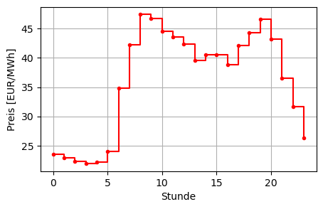

Wir lösen das LP in Pyomo mit einer Indexmenge zum Indizieren der Entscheidungsvariablen und Nebenbedingungen, vgl. Pyomo: Sets:

Code

model = pyo.ConcreteModel()

# Add the set of times to the model. This set will be used to index the variables:
model.T = pyo.Set(initialize=times)

# Add the variables to the model: energy (MWh) x_t produced in each hour
# include bounds on the variables: 0 <= x_t <= 100
model.x = pyo.Var(model.T, bounds=(0, 100))

# Add the objective function to the model including the sense of the optimization:
model.revenue = pyo.Objective(expr = pyo.quicksum(model.x[t]*prices[t] for t in model.T),
                              sense = pyo.maximize)

# Add the total energy constraint to the model:
model.resource = pyo.Constraint(expr = pyo.quicksum(model.x[t] for t in model.T) <= 1000)

# Add the constraints for ramping up: The @ decorates 
# the ramp_up function as constraints for all times of the set model.T.
@model.Constraint(model.T)  
def ramp_up(model, t):
    if t >= 1:
        # return the constraint expression:
        return model.x[t] - model.x[t - 1] <= 20
    else:
        # skip this index:
        return pyo.Constraint.Skip

# add the constraints for ramping down:
@model.Constraint(model.T)
def ramp_down(model, t):
    if t >= 1:
        # return the constraint expression:
        return -20 <= model.x[t] - model.x[t - 1]
    else:
        # skip this index:
        return pyo.Constraint.Skip

# model.pprint()

If you want to know what a decorator really does read for example this primer on decorators.

Code

# Let's solve the model:

solver = pyo.SolverFactory('cbc')
# solver = pyo.SolverFactory('glpk')
# solver = pyo.SolverFactory('appsi_highs')
# solver = pyo.SolverFactory('gurobi')

results = solver.solve(model, tee=False)
print(results.solver.status)

ok

Code

# Print the optimal revenue:
print(f"optimal revenue = {pyo.value(model.revenue):.2f} EUR")

optimal revenue = 42932.40 EUR

Code

# optimal production schedule x_t as a dictionary with the times as keys:
sol_dict = model.x.extract_values()
sol_dict

{0: 0.0,
 1: 0.0,
 2: 0.0,
 3: 0.0,
 4: 0.0,
 5: 0.0,
 6: 20.0,
 7: 40.0,
 8: 60.0,
 9: 80.0,
 10: 100.0,
 11: 100.0,
 12: 100.0,
 13: 80.0,
 14: 70.0,
 15: 50.0,
 16: 40.0,
 17: 60.0,
 18: 80.0,
 19: 60.0,
 20: 40.0,
 21: 20.0,
 22: 0.0,
 23: 0.0}

Code

# plot of the optimal production schedule:
plt.figure(figsize=(5, 6))
plt.subplot(2, 1, 1)
plt.step(times, prices, where='post', marker='.', color='red')
plt.xlabel('Stunde')
plt.ylabel('Preis [EUR/MWh]')
plt.grid(True)

plt.subplot(2, 1, 2)
plt.step(times, [sol_dict[t] for t in times], where='post', marker='.', color='green')
plt.xlabel('Stunde')
plt.ylabel('Erzeugung [MWh]')
plt.grid(True)

plt.tight_layout()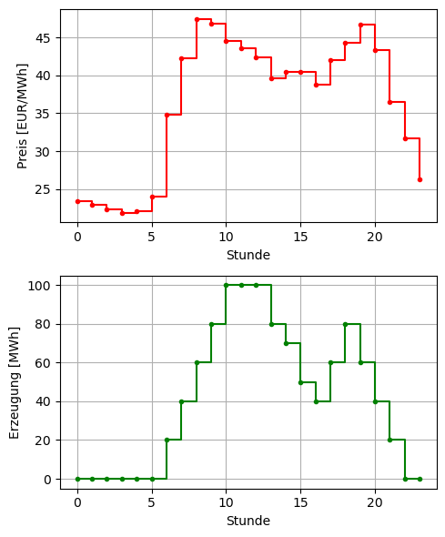

Code

# Alternative plot of the optimal production schedule 
# as a pandas dataframe with the times as index:
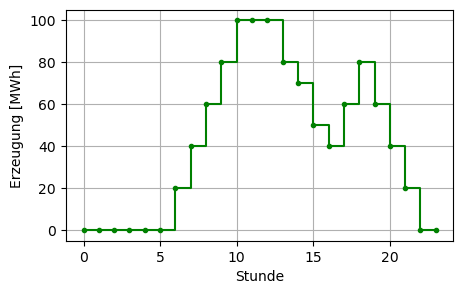
df = pd.DataFrame.from_dict(sol_dict, orient='index', columns=['x'])
display(df)

df.plot(drawstyle="steps-post", figsize=(5, 3), legend=False, color='green',
        xlabel='Stunde', ylabel='Erzeugung [MWh]', marker='.', grid=True);

	x
0	0.0
1	0.0
2	0.0
3	0.0
4	0.0
5	0.0
6	20.0
7	40.0
8	60.0
9	80.0
10	100.0
11	100.0
12	100.0
13	80.0
14	70.0
15	50.0
16	40.0
17	60.0
18	80.0
19	60.0
20	40.0
21	20.0
22	0.0
23	0.0

Hinweise

Pyomo und die Pyomo Dokumentation sind sehr umfangreich. Wir verwenden davon nur einen Teil, z. B. nur die sogenannten konkrete Modelle und keine abstrakten Modelle.
Unter Pyomo kann man den Größen Einheiten geben und so die Ausdrücke auf Konsistenz bzgl. Einheiten prüfen lassen, siehe Units Handling in Pyomo.

Übung

Lösen Sie das folgende lineare Programm (LP) mit Pyomo, d. h.:

Bestimmen Sie die Entscheidungsvariablen inklusive Einheiten, Datentyp und Schranken.
Formulieren Sie die Zielfunktion und die Nebenbedingungen.
Modellieren Sie das LP mit Pyomo.
Lösen Sie das LP mit verschiedenen Solvern, und geben Sie die Lösung formatiert aus.
Interpretieren Sie die Lösung! Ist sie plausibel? Ändern Sie z. B. die Daten, um Ihre Lösung an einfachen Spezialfällen zu überprüfen.

Gasoline-Mixture Problem: A gasoline refiner needs to produce a cost-minimizing blend of ethanol and traditional gasoline. The blend needs to have at least 65 % burning efficiency and a pollution level no greater than 85 %. The burning efficiency, pollution level, and per-ton cost of ethanol and traditional gasoline are given in the following table:

Product	Efficiency [%]	Pollution [%]	Cost [$/ton]
Gasoline	70	90	200
Ethanol	60	80	220

Quelle: Sioshansi, Ramteen; Conejo, Antonio J. (2017): Optimization in Engineering: Models and Algorithms. 2017, Springer. Seite 24 f.