Thermischer Speicher

Problemstellung

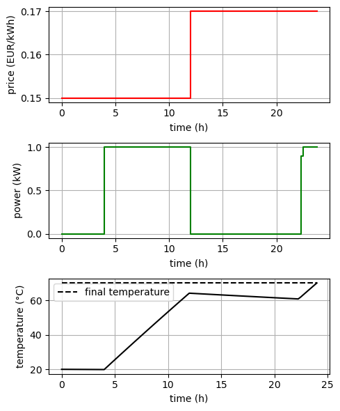
Sie wollen Ihren 150 Liter Warmwasserboiler aus dem Abschnitt Thermische Speicher mit den zusätzlichen, unten angegebenen Parametern kostenoptimal betreiben. In den kommenden 24 Stunden soll er von 25 °C auf 70 °C aufgeheizt werden. Der Strompreis beträgt in den ersten 12 Stunden 0,15 €/kWh und in den zweiten 12 Stunden 0,17 €/kWh. Wir bestimmen die optimale Ladeleistung in Viertelstundenintervallen.

import numpy as np
import matplotlib.pyplot as plt

# time:
T  = 24.0  # h
dt = 0.25  # h
n = int(T/dt)  # number of time periods
times = np.arange(start=0, stop=T + dt, step=dt)
periods = np.arange(start=0, stop=T, step=dt)
time_indices   = range(n + 1)  # 0, 1, ..., n - 1, n
period_indices = range(n)      # 0, 1, ..., n - 1

# thermal storage:
c = 0.175       # kWh/K
k = 0.0012      # kW/K
T_env = 15      # °C
E_max = c*75    # kWh, 75 °C
p_max = 1.0     # kW
E_start = c*20  # kWh, 20 °c
E_end = c*70    # kWh, 70 °C

# prices in EUR/kWh:
price = np.zeros(n)
price[0:n//2] = 0.15
price[n//2:n] = 0.17

plt.figure(figsize=(5, 2))
plt.step(periods, price, where='post', color='r')
plt.xlabel('time (h)')
plt.ylabel('price (EUR/kWh)')
plt.grid()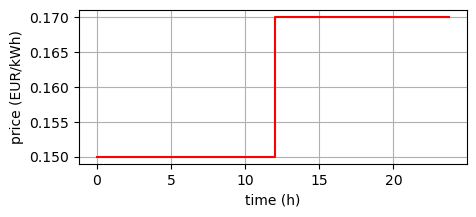

Modellierung

Daten:

• \(c_j\): Strompreis in €/kWh während der Zeitperioden \(j = 0, 1, \ldots, n - 1\)
• Parameter des Warmwasserboilers, vgl.Code Code oben und Abschnitt Thermische Speicher.

Entscheidungsvariablen:

• \(p_j\): elektrische Leistungsaufnahme des Warmwasserboilers in kW während der Zeitperioden \(j = 0, 1, \ldots, n - 1\) mit \(0 \leq p_j \leq p_{\max}.\)
• \(E_i\): Energieinhalt des Wassers zu den Zeitpunkten \(i = 0, 1, \ldots, n\) mit \(0 \leq E_i \leq E_{\max}\).

Zielfunktion: \(\min \sum_{j=0}^{n-1} c_j p_j \Delta t\)

Nebenbedingungen:

• \(E_0 = c \cdot 20\) °C
• \(E_n = c \cdot 70\) °C
• \(E_{i + 1} = E_i e^{-\frac{k}{c}\Delta t} + \frac{c}{k}(1 - e^{-\frac{k}{c}\Delta t})(p_i + k T_\text{env})\) für \(i = 0, 1, \ldots, n - 1\)

Implementierung

import pyomo.environ as pyo

model = pyo.ConcreteModel()

model.I = pyo.Set(initialize=time_indices)
model.J = pyo.Set(initialize=period_indices)

model.E = pyo.Var(model.I, bounds=(0.0, E_max))
model.p = pyo.Var(model.J, bounds=(0.0, p_max))

model.obj = pyo.Objective(expr=
    sum(price[j]*model.p[j]*dt for j in model.J),
    sense=pyo.minimize)

model.initial_energy = pyo.Constraint(expr = model.E[0] == E_start)
model.final_energy   = pyo.Constraint(expr = model.E[n] == E_end)

@model.Constraint(model.I)
def energy_update(model, i):
    if i < n:
        return model.E[i + 1] == model.E[i]*np.exp(-k/c*dt) + \
        c/k*(1 - np.exp(-k/c*dt))*(model.p[i] + k*T_env) 
    else:
        return pyo.Constraint.Skip

solver = pyo.SolverFactory('cbc')
# solver = pyo.SolverFactory('glpk')
# solver = pyo.SolverFactory('appsi_highs')
# solver = pyo.SolverFactory('gurobi')

results = solver.solve(model, tee=False)
print(f"status = {results.solver.status}")
print(f"minimal cost = {pyo.value(model.obj):.2f} EUR")

status = ok
minimal cost = 1.49 EUR

Ergebnisse

E_sol_dict = model.E.extract_values()
E_sol = np.array([E_sol_dict[i] for i in time_indices])

p_sol_dict = model.p.extract_values()
p_sol = np.array([p_sol_dict[j] for j in period_indices])

plt.figure(figsize=(5, 6))
plt.subplot(3, 1, 1)
plt.step(periods, price, where='post', color='r')
plt.xlabel('time (h)')
plt.ylabel('price (EUR/kWh)')
plt.grid()

plt.subplot(3, 1, 2)
plt.step(periods, p_sol, where='post', color='green')
plt.xlabel('time (h)')
plt.ylabel('power (kW)')
plt.grid()

plt.subplot(3, 1, 3)
plt.plot(times, E_sol/c, color='black')
plt.hlines(y=E_end/c, xmin=0, xmax=T, color='black', 
           linestyle='--', label='final temperature')
plt.xlabel('time (h)')
plt.ylabel('temperature (°C)')
plt.legend()
plt.grid()

plt.tight_layout()